Project Category: Geomatics
Join our presentation
About our project
Deformation of a railway occurs during a boring operation when the borehole deforms, and shifts the ground material beneath the rails. This shift propagates up to the surface and moves the rail ties, which pulls the rails with it. If deformation is left unmonitored it could cause severe damage to the tracks, costing the drilling company and railway owners time and money.
The current method of rail deformation monitoring is by a conventional levelling loop, using a digital level and rod. This method, while accurate, can be cumbersome by measuring each point, with an observer, a rodman, and potentially two required train spotters. Our project looks to investigate the use of a laser scanning total station to perform the deformation monitoring. Our goal is to see if this method is safer, more cost effective, and more logistically efficient, while still meeting the required accuracy of 1.5 mm and frequency of twice daily measurements.
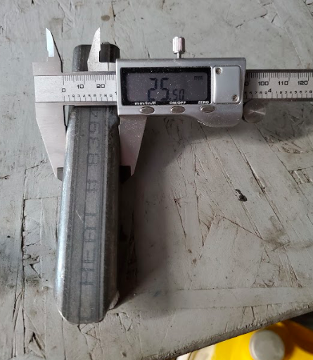
To do this, we performed a series of dynamic tests using a home-built railway model. The model was observed by a conventional levelling loop, and by laser scanner. The model was then deformed using a precisely measured item, and observed again. Data processing for the levelling loop was done using a spreadsheet, and data processing for the laser scanning was done in Trimble Business Center. A separate static test with the laser scanner was also performed to investigate the validity of this method under the conditions of an actual railway.
Meet our team members


Details about our design
HOW OUR DESIGN ADDRESSES PRACTICAL ISSUES
Safety
According to the Transportation Safety Board of Canada, between the years 2010-2019, there were 26 employee fatalities. During a pipeline operation, the railway that is being operated on is often not shut down during the drilling, meaning that trains can pass by at any time. To address this, railway owners have implemented strict safety rules when it comes to being on the tracks. These rules can cause large logistical issues in regards to getting clearance in a timely manner. The laser scanning solution allows for very minimal/no need for a person to be on the tracks. Unlike conventional leveling, the scanning process does not require a person holding a rod on the tracks. The only reason a person would need to be on the tracks is to remove rocks/debris from the scan area.
Fewer People
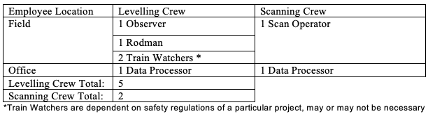
When it comes to the conventional method of rod and level observation(s) on a rail track, there typically needs to be 4 employees. One observer, one rodman, and two train watchers. For laser scanning however, there is no rod being observed, and since no people are on the track there is no need for train watchers. That means only one person operating the laser scanner is needed for our solution. Each method only requires one person in the office for data processing as well.
| Method | Field Crew | Office Staff | Total |
| Levelling | 4 | 1 | 5 |
| Scanning | 1 | 1 | 2 |
Observation Frequency & Efficiency
Typically during a drilling operation, monitoring of the railway is needed twice daily, once in the morning and once in the afternoon. Thankfully, the laser scanning method is able to reach this requirement. In our field test from 15 scans the average time of observation was approximately 15 minutes. This is not dependent on how many points of interest there are. For example if there were 10 points or 100 points of interest in the area we scanned, both cases would only take 15 minutes. Whereas with leveling, we averaged a time of 2.7 minutes/point observed. This means 10 points would take 27 minutes, 100 points would take 4.5 hours.
Observation Complexity
The method of laser scanning is actually quite straight-forward. Trimble has very simple instructions for a basic scan:
1) Select measure/scanning
2) Select the scan density
3) Enter the approximate target distance
4) Enter the required field of view
5) Capture a panorama image (select panorama checkbox)
6) Tap start
These are 6 steps that anyone can perform to generate a basic scan.
WHAT MAKES OUR DESIGN INNOVATIVE
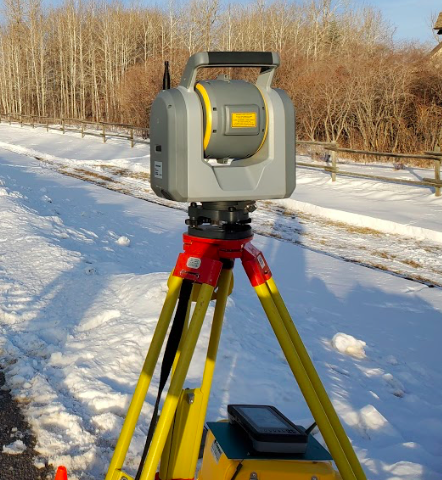
Hybrid Laser Scanning Total Station Approach
The Trimble SX10 is a combination of a laser scanner and a total station. Through our research, we are unaware of any other group that has attempted to use a laser scanning total station for a purpose like this.
One major benefit of using a hybrid device like the SX10 is it cuts down data processing time as points are automatically registered upon uploading them to a data processing software and do not need to be geo-referenced. In the field, the SX10 uses its total station functionality to be in orientation with known point(s) during the scan. Then when it is time for data processing, scans for each epoch are also in that orientation making the comparison process much simpler.
Areas Monitored Instead of Points
In a conventional levelling loop, points of interest along the track need to be set up in a control network such that those locations can be monitored. The location of these points needs to be stable throughout the entirety of the drilling process which could take weeks. Setting up those points can be tedious, and their spacing may not be adequate. For example, if the points are too spread out deformation may happen between the points but would never be observed.
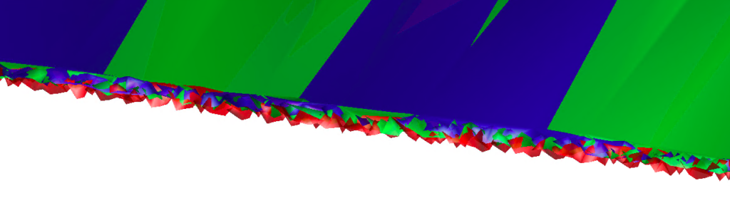
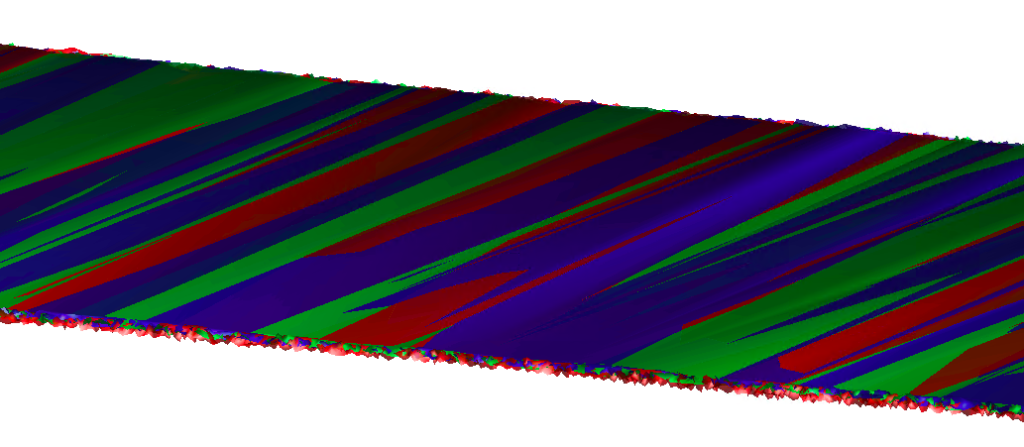
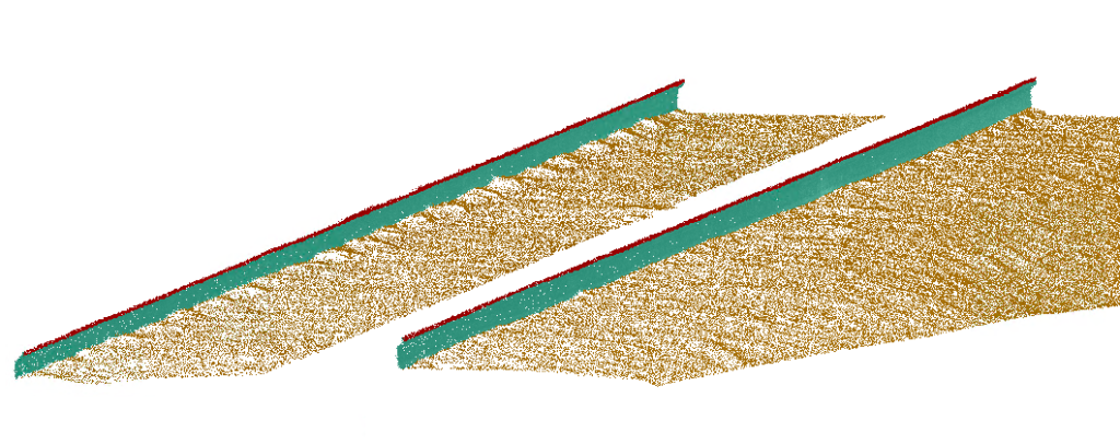
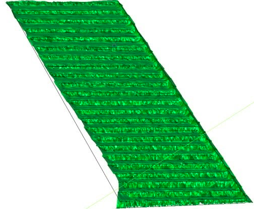
The laser scanning method however creates entire surfaces for comparison. These surfaces can be generated for an entire section of rail and a cut & fill grid comparison can be performed as shown on the left. This means deformations are more likely to be noticed at locations that aren’t specified by a point like in the leveling network.
WHAT MAKES OUR DESIGN SOLUTION EFFECTIVE
Field Work Simplicity
One of the most annoying things for a field crew is a complicated system/device. Thankfully, the use of a laser scanning total station provides observations with ease. Firstly, the total station portion of the SX10 is not far removed from a regular total station. This is the same with the scanning portion in comparison to regular laser scanners. There is not a steep learning curve and most manufacturers provide in-depth documentation, videos, and tutorials for all skill levels.
Effective Cost after A Certain Point
Through our research, we found that levelling requires a crew size of 5, and scanning requires a crew size of 2.
By way of first hand experience during our field test we have broken down the average times for the levelling and laser scanning.
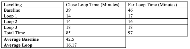
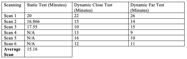
The baseline loop for levelling consists of three levelling loops that are then averaged for the best estimate of a baseline elevation; this is why the baseline is larger than the loops. The average loop time and the number of points observed can be used to calculate the time/point. With an average loop time of 16.17 minutes to observe 6 points (rail model points 1-6) the time per point is 2.70 minutes/point. The observation time using laser scanning has the luxury of not being dependent on the number of physical points observed. This means if a geotechnical report required a point on each side of the track to be measured every 0.25 m over a 10 m section of track it would take levelling around 1.8 hours, whereas with the scanner it would take approximately 15 minutes. With this logic, the knowledge of crew size requirements, and the wage of each crew member as shown in the table below, a pointwise analysis can be performed.
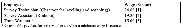
After entering the data into our levelling loop data processing sheet, we have found that it takes about 5 minutes to copy 6 points from paper levelling loop observation sheets into the spreadsheet. This results in a processing speed of 0.833 minutes/point for levelling. For laser scanning, we have found it takes us approximately 20 minutes to generate and compare one surface by the cut-fill method, and each isolation check measurement takes approximately 5 minutes. If we assume that the person processing the data gets paid the same $24.68/hour then we can analyze the total cost of each method per point measured based on observation and data processing cost, as shown in the figure below.
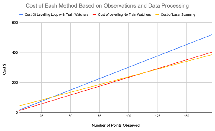
The figure above shows us the cost comparison for observations and data processing for levelling with train spotters, levelling without train spotters needed, and laser scanning. From this we can see that laser scanning is more cost-effective after 35 points have been observed if the project were to require train watchers. It becomes cost effective to use laser scanning after 114 points if the project does not require train spotters.
Logistically Effective
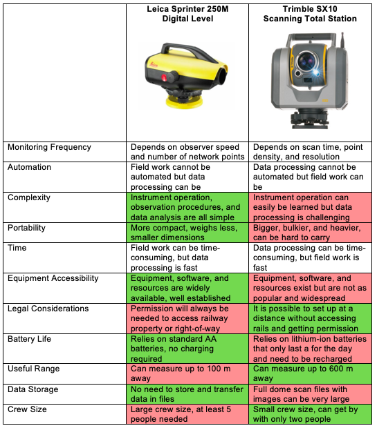
When comparing logistical components of conventional levelling and laser scanning there are many considerations such as: monitoring frequency, automation potential, complexity, portability, time, equipment accessibility, legal considerations, battery life, useful range, data storage, and crew size. While this list is long, depending on the project these factors may play a major role. The table summarizes and compares the logistical effectiveness of each method.
HOW WE VALIDATED OUR DESIGN SOLUTION
Dynamic Test
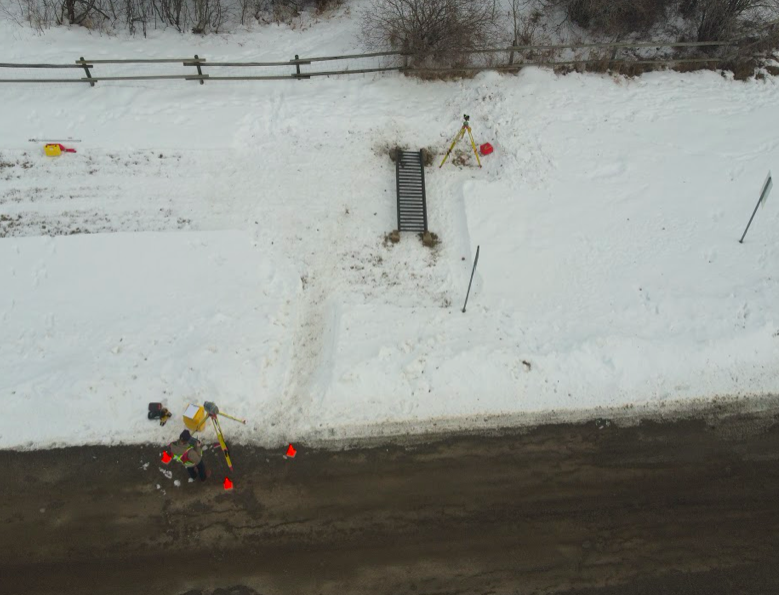
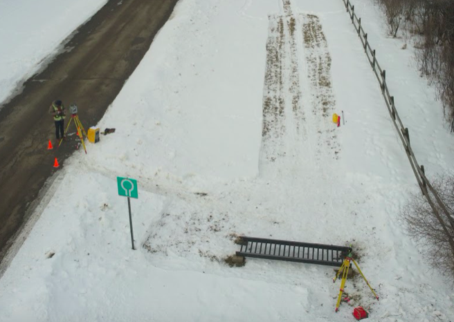
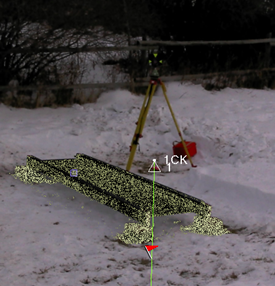
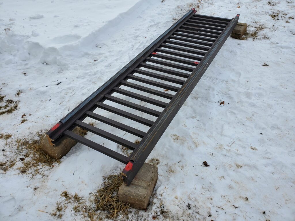
One of the ways we validated our solution was a dynamic field test. This was performed on an acreage in Okotoks. To do this a home built railway model was constructed using a deck railing and strips of angle iron, as we needed a device to deform the rails.
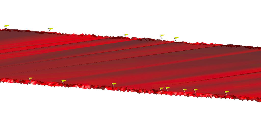
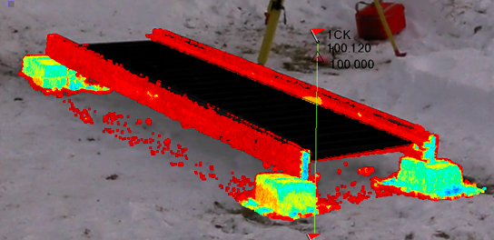
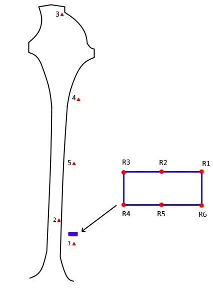
The railings were 3 metres long and 0.8 metres wide. Two pieces of 1.5” x 1.5” x 0.125” angle iron were used to simulate the rails on an actual track as the laser scanner may return different results when scanning metal as opposed to wood. The angle iron was affixed to the tracks using wood screws through holes that were drilled in the angle iron. Six drywall screws were screwed into the track wood and were left approximately 1.5 cm above the surface of the wood so that a levelling rod could be held on them. These drywall screws are the rail points (R1-R6) that were observed during the levelling loops on the tracks. The image on the right shows these points as red marks.
A control network was set up in the cul-de-sac and ditch west of Elliott’s acreage. Five control points were established. The control points that were on the asphalt (1 and 2) were 2” concrete nails with flagging that were left above the asphalt approximately 1 cm to ensure that a levelling rod could be used on them. The control points in the ditch were ~10” long pieces of rebar with rounded tops and punch marks on the top to make it easier to centre the equipment on the points, which were left above the ground by a few centimetres for the same reason as the concrete nails.
Points 1-6 are the network control points, whereas points R1-R6 are the rail model points.
Conventional Levelling
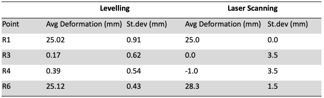
In total, 12 levelling loops were performed on the rail model in groups of 6. Of the 6, the first 3 before deformation were adjusted, averaged, and used as a baseline. After deformation, 3 loops were compared to the baseline and used to find the mean deformation of points R1-R6. This test was performed as a comparison for the laser scanning results. We know the levelling method works, as it is the current professional standard for this type of deformation monitoring; and we can see how the scanning results match up.
Laser Scanning
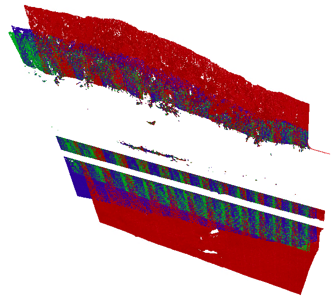
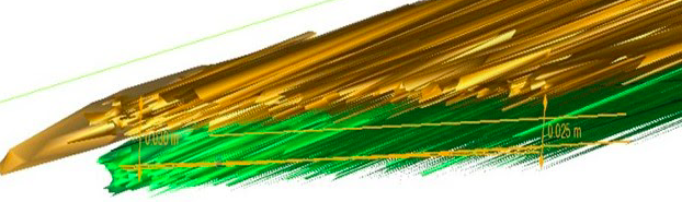
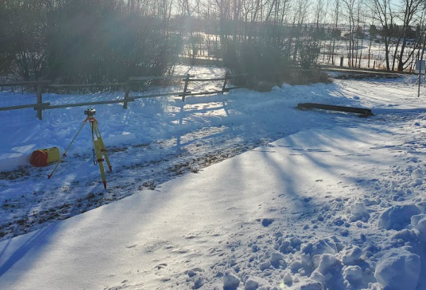
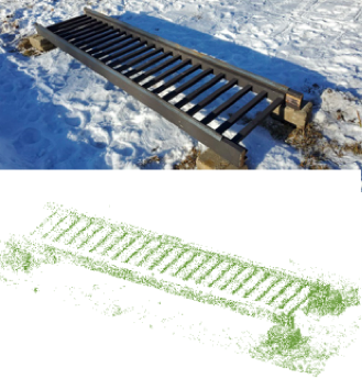
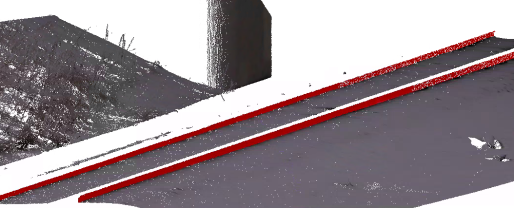
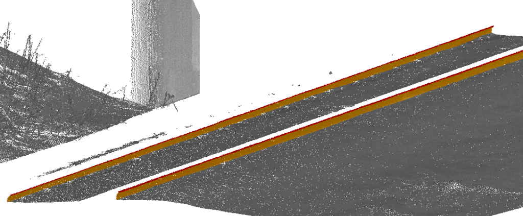
Two types of test were performed with the laser scanner: a close test, and a far test. For the close test, the scanner was set up on point 2 about 9 metres away from the model. Coordinates of points 1, 2, 4 were entered into the data collector, point 4 was back-sighted, and point 1 was used as a check shot. The scans were then performed, 3 before deformation, and 3 after. In the far test the scanner was set up on point 3, point 1 was the backsight, and point 4 was the check shot. These scans proved to not be useful as the distance was about 114 metres away, the scanner could really only see the north face of the tracks and only record about 21,000 points as opposed to the close tests 550,000 points.
Static Test
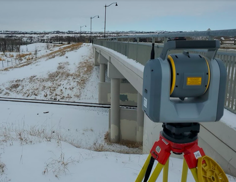
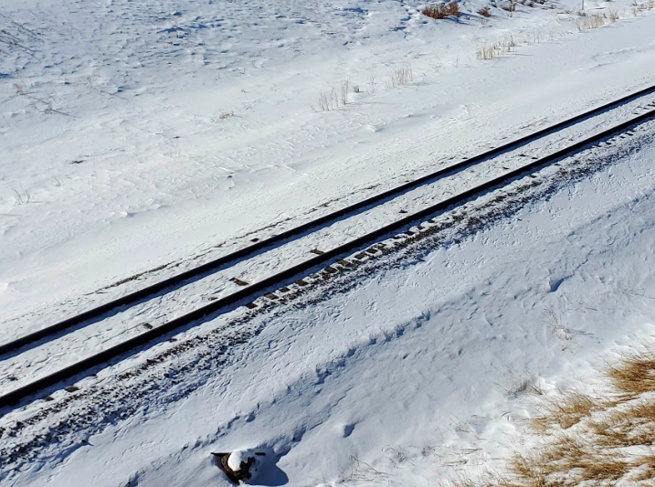
A static test was performed on an actual railway track in Okotoks, Alberta. Measurements still could not be performed directly beside the tracks due to safety regulations. Instead, the scanner was placed higher up on an embankment looking down on the tracks. Three scans were performed with the purpose of investigating the method’s validity on an actual track (i.e. How will the scanner perform with the actual track materials and geometry? Will we obtain a good scan return?). This test also helps us determine our solution’s precision; after processing no deformation should be observed, as the rails are not expected to move in that short time frame.
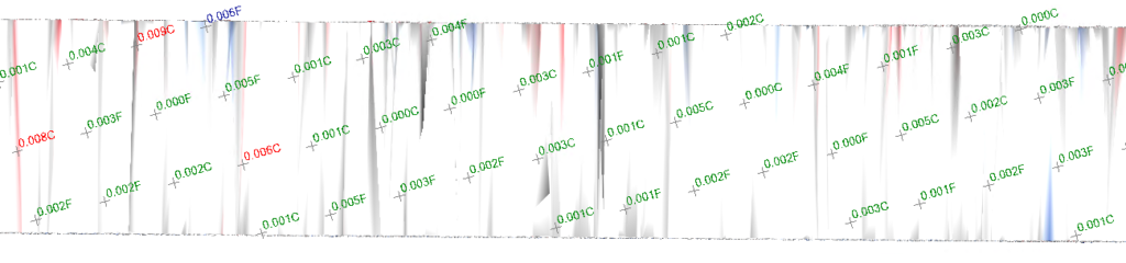
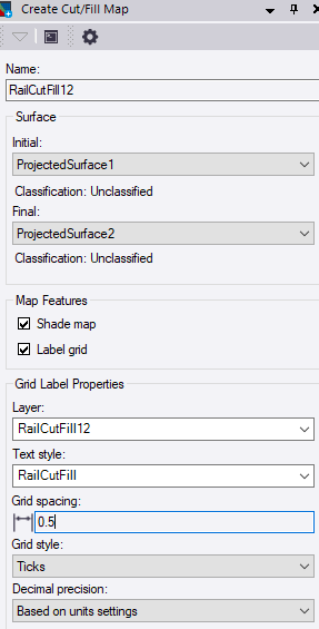
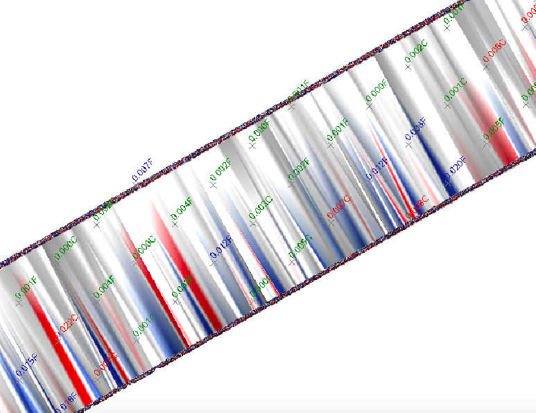
This static test allowed us to compare multiple scans to a reference scan. This was done by creating a cut-fill map in Trimble Business Center. The numbers on the grid show the elevation differences between a monitoring scan and the reference scan. Our main takeaways from the static test is that: Other than a few outliers, the cuts and fills are small enough to consider no deformation being detected. The scanning method can detect if the rails remain stationary to an acceptable margin considering the scanner’s manufacture precision.
FEASIBILITY OF OUR DESIGN SOLUTION
It Is Not Feasible…
For our solution to be feasible in industry we required 3 main requirements to be met:
1) Accuracy: The method should be accurate to under 1.5 mm.
2) Safety: No person should need to be on the track at any time.
3) Cost Effective: The cost of the method should be on par, if not cheaper than leveling.
Requirements 2) and 3) have in some sense been met:
2) Safety: Other than removing any debris from the rails no person has to be on the track during the actual observation process.
3) Cost: In certain scenarios, laser scanning becomes more cost effective than leveling. This is dependent on the number of points.
– If train watchers are required then laser scanning costs less after 35 points are observed.
– If no train watchers are required then laser scanning costs less after 114 points are observed.
Requirement 1) however has not been met.
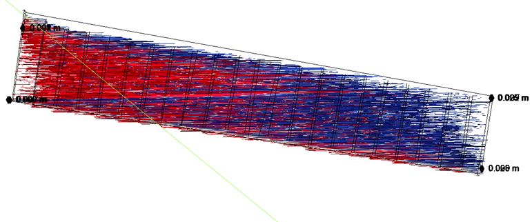
From our investigation in the dynamic test, it was found that 3 of the 4 isolation point measurements we calculated had a standard deviation equal to or greater than 1.5 mm. Also shown in the image below, when the cut-fill method is used we can see deformations of 31 mm being measured when the expected deformation was 25.5 mm. This is an inaccuracy of 5.5 mm; 4 mm over our limit.
Accuracy is the most important requirement for a method to be deemed feasible. Due to the results previously described, the inaccuracy of this method has proven it to be infeasible.
Additionally, the logistics of the scanning method may be too inadequate given a user’s specific scenarios. Examples of these logistical issues are:
– The steep learning curve for processing point clouds.
– The equipment is bulky, and if the project is off the beaten path, carrying it everywhere may be tiring.
– The equipment/Software is available but not a staple in all surveying firms.
– The lithium ion batteries of the scanner will only last one day without being charged.
– The data file sizes from the scanner can be very large, especially with full dome scans.
More Research Required…
While not viable currently, we believe this could be a viable method in the future as software and scanners are further developed. Some opportunities for additional investigation include:
– Data processing with a different software. We used Trimble Business Center due to its availability but maybe there is another software more suited to point cloud processing.
– Field work with a different scanner. There are many scanners made by various different companies. We used the Trimble SX10 but another model or brand could be investigated.
– A different method of processing. Our team used a cut & fill method that compared a baseline surface to the deformed surfaces. As a group we have had no prior experience with laser scanning, but saw this as our best approach. There could be more advanced methods known by more experienced individuals.
Partners and mentors
We would like to extend a major thank you to our project advisor Dr. Robert Radovanovic. Without his guidance this project would not have been possible. We would also like to extend acknowledgement, and thanks to some members of the professional Geomatics community who took time out of their day to be interviewed by us: Wade Bowley, Tomasz Stefanczyk, Lucas Cairns, Ryan Deighan, Logan Ceretti, Brett Watson, and Nathan Sikkes.
Our photo gallery