Project Category: Petroleum
Join Our Presentation
We will be here from 10:00am to 12:30pm on Tuesday, April 13.
Our Project
This project focuses on the reservoir characterization of the Cadomin formation in township 66, located southwest of Grand Prairie in Alberta. The Cadomin formation is deposited in the Early Cretaceous era and is a continuous tight gas accumulation reservoir that spans across British Columbia and Alberta. The purpose of the project is to select and propose the drilling operation for 4 new wells within this township based on the knowledge we have on the reservoir. These new wells will be evaluated through reservoir modelling and production forecasting to determine if the new wells have a positive economic outlook.


Our Design
1. BACKGROUND
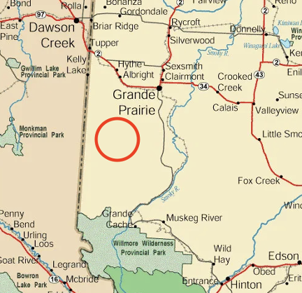
The Cadomin formation is a large continuous tight gas accumulation reservoir, which is characterized by thin net pays and tight rocks containing hydrocarbons that span across a large area. The Cadomin formation spans across western Alberta, reaching as far as British Columbia. Due to size of this formation, the analysis of the Cadomin reservoir for this project will be performed within the township square 066-10W6, which is located southeast of Grand Prairie in Alberta.
Geological and contour maps for the Cadomin formation in township 66 can be found in the photo gallery.
More details can be in seen in the sub-sections below.
1.1 Cadomin Formation
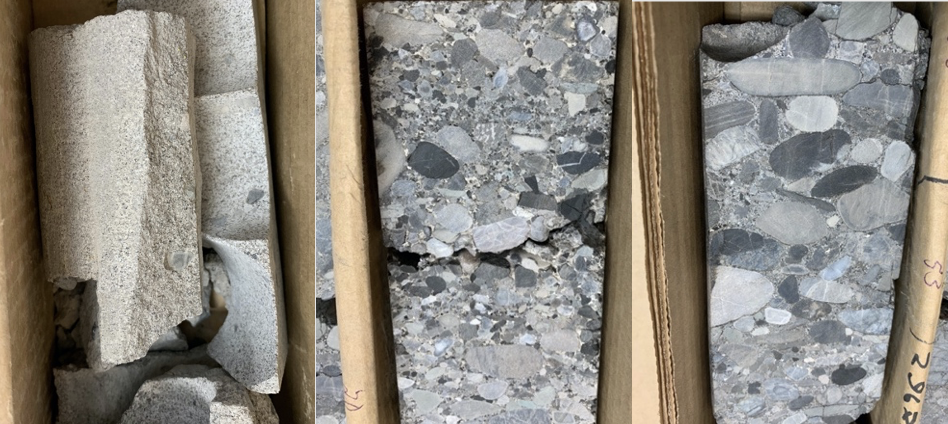
The Cadomin Formation was deposited in the Early Cretaceous Period to the east of the Rocky Mountains, close to the border of what is now Alberta and British Columbia. The primary rock type found within the Cadomin Formation is poorly sorted conglomerates due to the nature of a fluvial deposit in a high energy depositional environment.
The trapping system for the gas in the Cadomin formation is an updip hydrodynamic trap, where despite the density differences, the water is located above the gas acting as the seal. The water remains above the gas as a trap due to the small pore sizes and capillary pressure forces experienced by the gas and water. This prevents the water from displacing the gas below it.

1.2 Pool History
From the 188 wells drilled to date in the township, 40 are commingled and target eight plays: the Peace River (Cadotte and Paddy members), Spirit River (Falher and Notikewin members), Bluesky, Gething, Cadomin and Nikanassin formations.
The pressure history within the Cadomin formation varies due to the nature of the continuous tight gas accumulation. Producing wells may not impact the pressure of other Cadomin producing wells as they may not communicate with each other due to the low permeability. The formation pressure historically ranges from 2,900 to 3,500 psi.
2. CORE AND LOG ANALYSIS
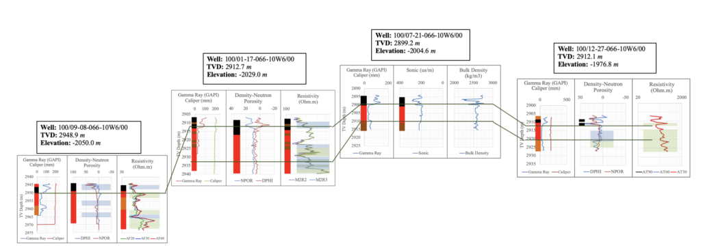
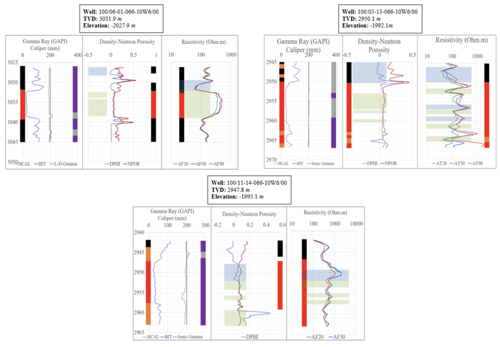
Core data and well logs were studied to provide a better understanding of the reservoir, and to aid in the characterization of the reservoir. Well logs helped us to picture the thickness, stratigraphic layers and the fluid content in Cadomin; while core data helped us to correlate rock properties to the parameters measured with wireline logs. From the correlations between core data and well logs, we were able to determine several important reservoir properties such as permeability, porosity, gas and water saturations, net pay zones and other geomechanical parameters.
Raster well-logs were available for all of the existing wells drilled in the township. Using gamma ray, caliper, sonic and resistivity logs, we were able to identify the fluid and sedimentation layers in each well, and build several cross-sections from there. The values plotted on these logs were extracted into LAS files which then helped us to calculate and extrapolate reservoir properties for all wells.
The core data for Cadomin formation were only available for well 05-13 and well 05-30. The analysis focuses on examining the relationship between the porosity and permeability data from core versus those from the logs for wells 05-13 and 05-30, and establish a correlation that can be used to calculate other reservoir properties for wells that only have well logs.
More details can be in seen in the sub-sections below.
2.1 Log Analysis
Open-hole well logs, mainly gamma gay, caliper, density and neutron porosity, and resistivity logs, were interpreted for several wells in the cross-sections of A-A’, G-G’ and various wells near the edge of the township.
Gamma ray logs are typically used to identify lithologies in the formation, specifically for sandstone and shale due to the distinguished GAPI values for each of those lithology. For instance, GAPI for sandstone is typically within 15 to 30, GAPI for shale is between 115-130. A caliper log is used to measure the bore-hole dimensions, and by comparing the caliper log values to bit size, mud cake and sloughing can be identified. If the caliper value is less than the bit size, it suggests that mud cake exists in that interval, while the opposite is true for sloughing. The density-neutron porosity log is helpful in identifying lithologies and fluids (gas, oil or water) in the formation. They are shallow reading logs and may be impacted by the presence of drilling mud. A resistivity log typically has 3 readings at different traces (shallow, medium, deep). The deep trace (AT90) is used primarily to identify lithologies and potential hydrocarbon zones since the deep trace reads the uninvaded zones unaffected by drilling of the formation.
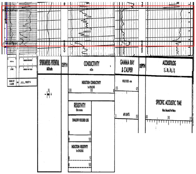
More cross sections and log interpretation plots can be found in the photo gallery.
The logs analysis was compared with the data collected from core analysis to ensure that the logs were corrected and calibrated with respect to the core before conducting net pay calculations. Once the log readings have been correlated, the same correlation was applied to all other wells in the township. The logs were interpreted from the aspect of water saturation, shale volume, porosity and cut-offs for net pay (values can be found in the photo gallery). Core calibrated values were used instead of the raw value from the logs.
2.2 Core Analysis
Core porosities for both 05-13 and 05-30 were plotted against bulk density and sonic transit time. Both the sonic transit time and bulk densities were used for this correlation as they provide good indications of the lithology in the reservoir. The core porosities from the bisecting line equation were compared to log porosities and the log depths were shifted to match the core porosities as the core is assumed to be a better representation of the formation. This correction was carried out for each depth interval once the trend was identified. Other methods of log-core calibration such as core gamma rays were not used to correct the log depths to the core depths as they were not available for the core samples. Detailed analysis can be found in our ENPE 511 Final Report.
The core data was plotted on a porosity-permeability cross plot to determine the rp35 pore throat aperture. Identifying the pore throat aperture helps determine the distinctive flow unit for the tight-gas reservoir. A flow unit is a reservoir characteristic that depends on porosity and permeability; this is used to gauge fluid flow in the reservoir based on similar pore types. The pore throat chart also helps to estimate initial production rates depending on the flow unit. These plots show that the permeabilities in the Cadomin formation fall predominantly under the mesoport and macroport pore-size classes which are in the ranges of 0.5 μm to 2.5 μm and 2.5 μm to 10 μm, respectively. Since permeability is proportional to flow rate, the conclusion can be made that the two flow units show that there are two different rock types in the formation which aligns with the analysis on the pore-throat aperture plots as well.
The relative permeability is a dimensionless measure of the flow preference of the porous medium for one fluid phase versus the other fluid phases present in the rock and is affected by pore size distribution. It is calculated as the ratio of the effective permeability of the fluid to the absolute permeability of the rock. The relative permeability values were calculated using Corey’s correlation.
Capillary pressure is the pressure between two immiscible fluids in a tube as a result of the interaction of forces between the fluid and the tube walls (Aguilera, 1990). For a reservoir, the capillary pressure is the pressure hydrocarbons experience inside of a pore throat as a result of the pore size and fluid interactions. Therefore, the smaller the pore throat, the larger is the capillary pressure.
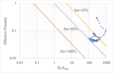
As for water saturation analysis, the well-known Archie’s equation cannot be used for our formation due to the presence of shaly sand. Instead, the Poupon equation which provides a correction for water saturation based on the presence of laminated shales. The formation water resistivity (Rw ) in the above equations was obtained from the Canadian Well Logging Society (1987) database and corrected for the temperature in the formation. From the Pickett Plot shown here, there is no uniform distribution of SW values in the reservoir, which further proof that the Cadomin formation is highly heterogenous.
3. FLUID ANALYSIS
The fluid analysis was conducted from the aspect of fluid properties (pressure, volume and temperature) and composition of the reservoir fluid. Because the reservoir is a dry gas reservoir, the only fluid that can be produced from it is gas.
More details can be in seen in the sub-sections below.
3.1 Reservoir Conditions: Pressure, Volume, Temperature
The pressure and temperature of the formation at its initial state was determined to be 3090 psi and 85°F respectively from averaging the data from all the Cadomin wells. The temperature in the reservoir remains constant due to the depth underground and the lack of heat exchange to new temperature bodies. The averaged molar mass of the produced gas is 18.599 lbm/lbmol. This was calculated by using the mole fraction of the composition within the gas. The gas density was determined using the real gas law and the corresponding compressibility factor. At the original reservoir conditions, the gas compressibility factor is 0.8726 with a gas formation volume factor of 0.0051 CF/SCF, gas density of 9.519 lbm/CF and viscosity of 0.199 cP.
3.2 Fluid Analysis
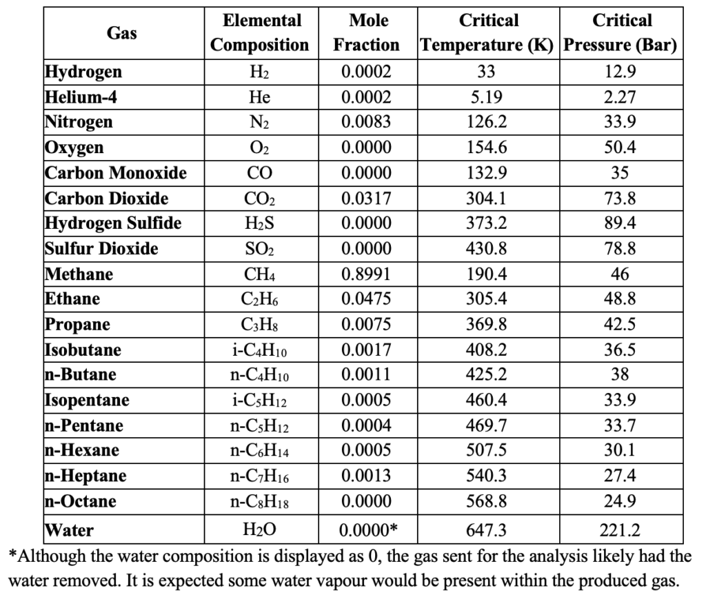
The Cadomin formation is a dry gas reservoir. This is reinforced by the lack of oil production in the Cadomin producing wells within the township. A minimal amount of water is occasionally produced from the Cadomin wells ranging from a cumulative total of 3,000 bbl to 19,000 bbl for the entire lifespan of a well. This is due to the water contained within the gas that condenses out when it reaches surface temperatures. There is no hydrogen sulfide gas produced from the Cadomin wells, but the gas is still considered to be sour due to the presence of carbon dioxide (CO2). It is important to note that the Cadomin wells produces an average natural gas composition of CO2 at 3.17% with a range of CO2 composition from 1.25% to 4.24%. The full gas composition is shown here.
4. PRELIMINARY ESTIMATIONS
In the earlier stages of this project, estimations were calculated for the reservoir reserves and forecasted production for the wells that are producing from the Cadomin formation. The volumetric reservoir reserves, or Original Gas-In-Place (OGIP) were calculated using the porosity-saturation-net pay map. As for production forecasting, decline analysis was conducted on the wells of interest first to model the production trend before extrapolating the trend to estimate the gas production for the future. Type Wells were also used as another evaluation/estimation method to predict the production from historical data of other wells with similar properties.
More details can be in seen in the sub-sections below.
4.1 Original Gas In Place (OGIP)
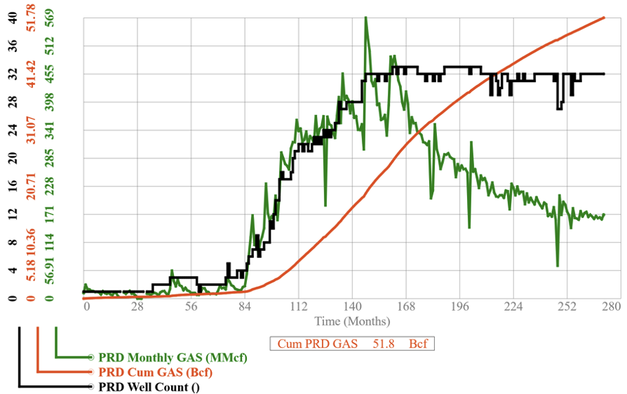
The volumetric reserves have been calculated from the porosity-saturation-net pay map. The surface area of each layer has been measured using Digimizer. The calculated original gas in place (OGIP) was estimated at 262.2 BSCF, where the formation factor is 0.0051 ft3/SCF. Of the overall cumulative gas that has been produced from this township (51.8 BSCF) this represents a recovery factor for the entire township of 19.76 %.
4.2 Decline Analysis
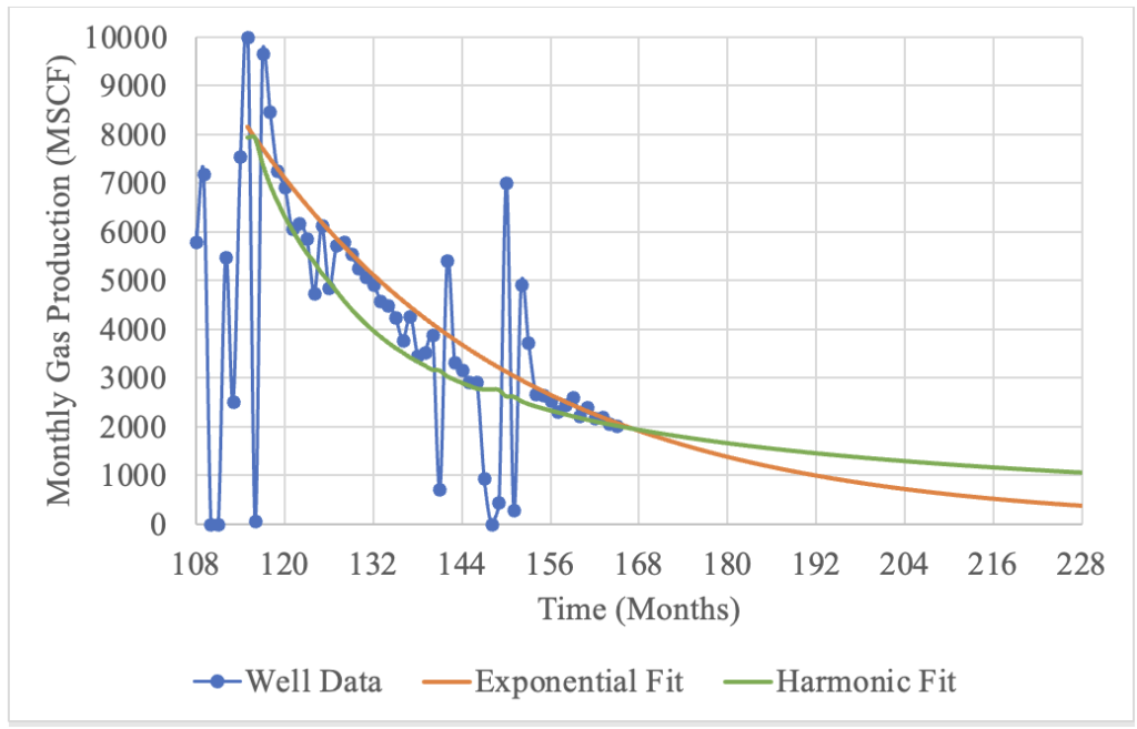
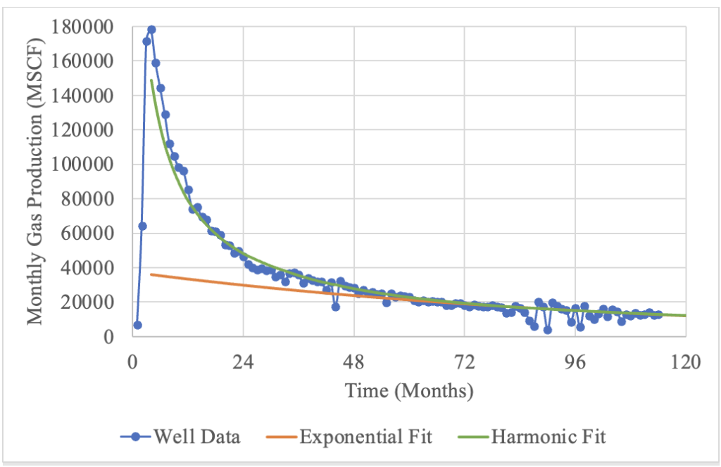
Decline analysis was performed on the vertical producing wells 05-13 and 11-14. Exponential and harmonic curves were extrapolated on the production data to determine the best fit for these wells. It is assumed that there have been no changes in operating conditions during primary production. This assumption may not hold as there are various points in production that appear to fluctuate. The reason for these fluctuations could not be determined as the well operator has not released this information as public knowledge, but it may be due to equipment repairs, valve or oil changes, workovers or new perforations. To lower errors from the assumption, the decline curves were formed with data past any large fluctuations, where the production data is most consistent and recent. Well 05-13 fits an exponential, while 11-14 fits a harmonic decline. The decline between each well appears to be independent of the other wells, despite their close distance. This further reinforces that the wells do not communicate fluids between each other. This is because it is expected that wells producing from the same reservoir that communicate the fluids would have a similar decline curve to neighbouring wells, but this is not the case. A decline curve was fit to the horizontal well 08-12. This was found to best fit a harmonic curve. The production for this horizontal well fits the shape expected as outlined in the drive mechanism, where the initial produced gas was very high and sharply decreases until it levels off at a very low production rate.
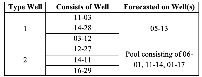
4.3 Type Wells
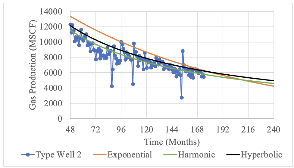
The production forecast and decline analysis can be done on a pool of wells using type wells. Several wells that have a similar reservoir properties, mainly permeability, to the well of interest have been grouped together as and is considered as a type well. The wells grouped and averaged for each type well are listed below. Production decline analysis was done on the averaged production rates of that type well to determine the decline constant and the decline curve that best fits the type well. The decline constant and decline curve are then applied to the wells of interest, for instance 05-13 for Type Well 1, to determine if the type well method can produce a reasonable forecast on those wells of interest which can then verify the type well is an acceptable forecast for future wells. A hyperbolic curve with b = 0.975 best fits the averaged production from Type Well 1, hence the same decline constant and curve from Type Well 1 was applied to the production from 05-13. A harmonic curve (hyperbolic curve with b = 1) has been determined for Type Well 2, and the harmonic curve and decline constant were fitted onto the group of 11-14, 06-01 and 01-17.
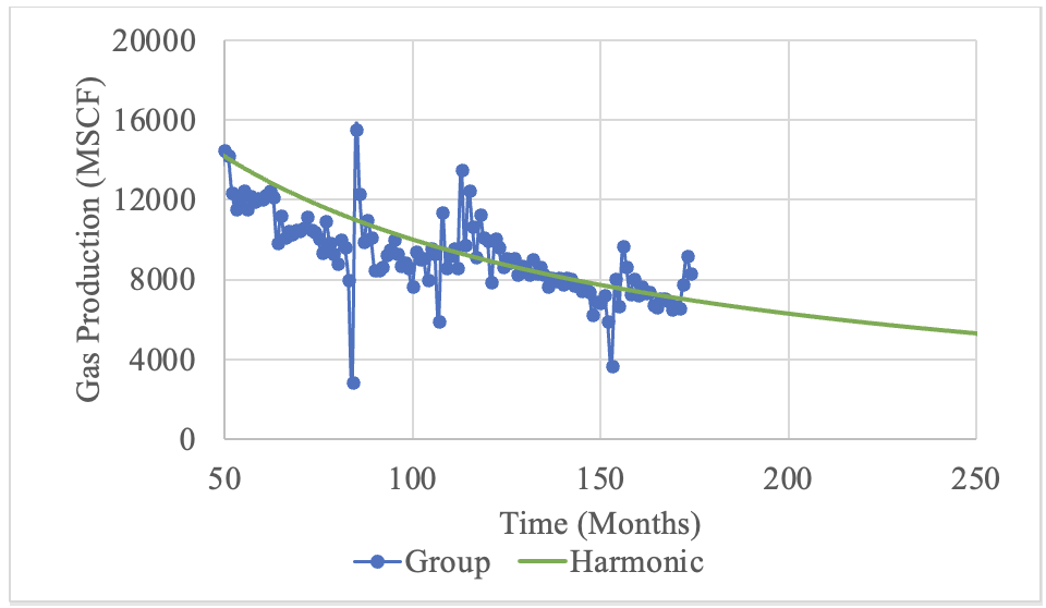
As there was only one horizontal well producing from the Cadomin formation, other Cadomin horizontal wells from outside the township were used for the type well. As many of these wells were outside of the township of study, it is assumed that the horizontal wells have similar properties to the area of proposed drilling. All of these wells produce directly from the Cadomin formation. The monthly production rate for each well was normalized to the total lateral length of the well to determine the production rate per foot. This rate was then averaged to create the type well forecast of the production per foot of lateral length. It can be seen from this horizontal type well forecast that a very large amount of gas will be produced initially in the first 12 months of production which then levels out by the 20th month. This phenomenon was previously described, it is due to the gas found in the fractures being produced quickly in the early stages of the well. Once this gas is produced, the gas trapped within the rock matrix slowly seeps out into the fractures which are then produced at a slower rate.
5. DRILLING AND COMPLETIONS
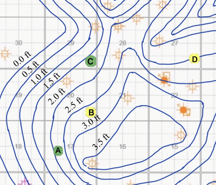
A total of 4 new wells will be drilled as part of the purpose of this project. Wells A and C are vertical wells, located in section 17 and section 29 respectively. Wells B and D are horizontal wells, located in section 20 and section 27 respectively. The drilling locations were selected based on composite consideration from the aspects of porosity, gas saturation, permeability and net pay zones. The drilling depths are elaborated in the following subsections, and are determined based on the depth of the Cadomin pay zone at each drilling location.
More details can be in seen in the sub-sections below.
For a more detailed analysis on the geomechanical properties of the formation, please join us at our Zoom Meeting room to learn more.
5.1 Well Site Designs
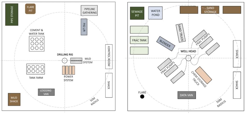
The drilling and flaring requirements for vertical and horizontal drilling are essentially the same, hence each well pad will have the following items as suggested in “Wellsite Spacing Requirements”.
The key elements needed on the well site include drilling rig, blowout prevent, shale shaker, wellhead, Christmas tree, frac fleet, flare pit, storage and control rooms. The proposed designs for drilling area and fracking are shown here.
5.2 Well Casing and Drilling Muds
Surface casing is included to provide sufficient shoe strength to drill through high-pressure zones. It is typically cemented to the surface. Surface casing must be set to a depth where it can prevent loose formations to cave in, a phenomenon that is often encountered at shallow depths. An intermediate casing is needed in horizontal well to protect the production from abnormally pressure zones in the formation above the pay zone and an additional layer of protection from pressure surges within the wellbore during production. Production casing is fitted to isolate the hydrocarbon zone from surface formation, and allows the formation pressure to be contained, especially during an event where there may be a leakage in tubing. A blowout preventer (BOP) will be fitted onto the conductor casing. This is to ensure that the unconsolidated formations or any unidentified groundwater sources can be isolated from the production.
Invert Oil Emulsion Muds (IOEM) will be used as the drilling fluid, with the addition of barite to provide the required viscosity. IOEM was selected instead of water-based muds as sloughing of shales may occur with presence of shaly sand in the Cadomin formation.
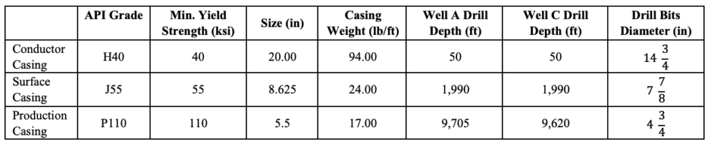
Tricone (roller-cone) bits were successful in producing good quality cuttings in the Nikanassin formation. As the Nikanassin sits below the Cadomin formation, and the planned total depth of well A and well C will reach the Nikanassin, roller-cone drill bits with IADC code 547 will be used for drilling the vertical wells.
Some of the potential drilling problems that could be encountered during drilling operations are identified on the well schematics in the sections below. Please join us at our Zoom Meeting room to learn more about the potential drilling problems and issues.
5.3 Horizontal Wells
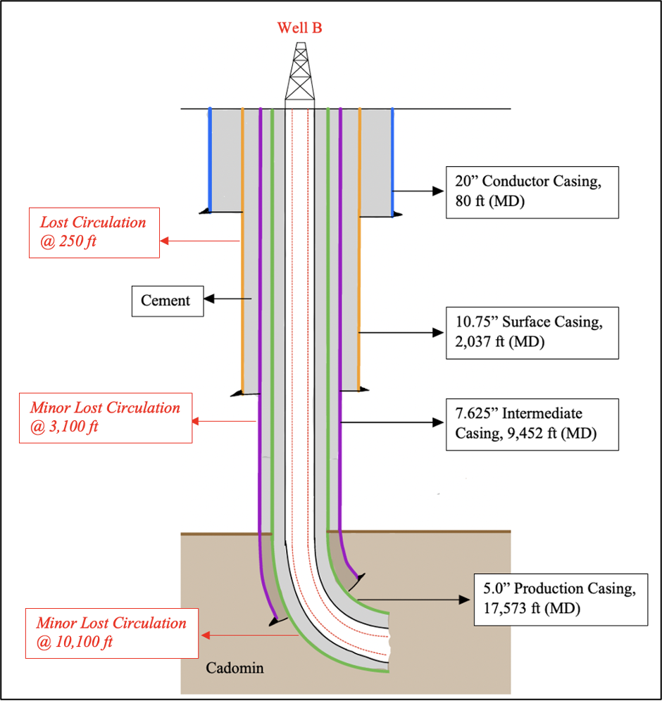
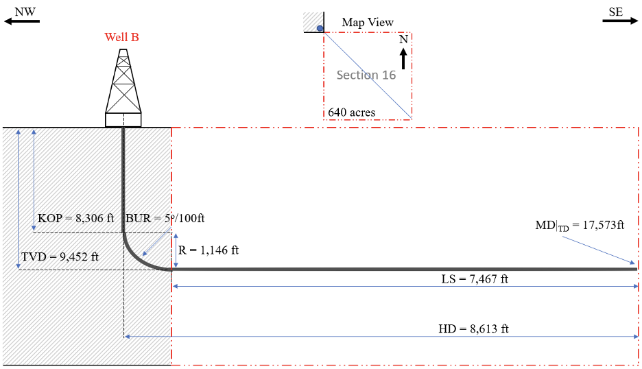
WELL DESIGN: WELL B
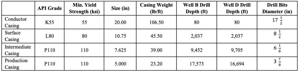
Well B must land at a depth of 9,452 ft at the top of the pay zone. The kick-off point (KOP) was calculated to be at 8306 ft in the Falher formation with a buildup rate (BUR) of 5°/100ft to minimize dogleg severity. Assuming a 640-acre lease, the well pad is placed in section 20: this allows for a lateral section (LS) reaching 7467 ft, which will be rounded to 7500 ft in length when drilled at a 135° azimuth. The measured depth (MD) at total depth (TD) would be around 17600 ft.
WELL DESIGN: Well D
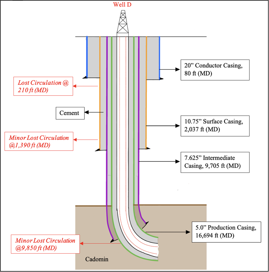
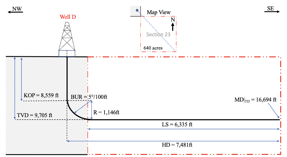
Well D should land at the top of the pay zone at 9705 ft. At a BUR of 5°/100 ft, the KOP for well D will be at the depth of 8,559 ft, with curve radius of 1,146 ft. The horizontal portion of the well will be drilled from the NW to SE of the township based on the formation top contour map. To minimize interferences from other wells along the lateral section, the lateral length of well D is determined to be 6,335 ft at an azimuth of 135°. The MD of well D at TD would be 16,694 ft.
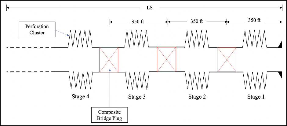
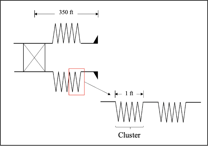
Hydraulic fracturing is one the most common and effective methods to increase production rates in tight gas reservoirs with low permeabilities. This well treatment can be implemented after perforations have been completed. The treatment uses slickwater, a water-based fluid mixed with low concentration of polyacrylamide (1 : 2000 of polyacrylamide to water), and proppants to increase fracture conductivity from 0.5 md-ft to 5.0 md-ft. Slickwater will be injected into the fractures at high rates to keep proppants suspended and allow the proppants to be transported deeper into the fractures. Plug-and-perf operation has the flexibility of altering distance between perforation clusters, the amount and the length of each cluster. Tubing Conveyed Perforation will be used as the primary tool for hydraulic fracturing perforation. The current best practice in industry, especially in tight gas and shale gas operations perforates 5 clusters at each perforation stage, at 6 shots/ft of shot density. There will be 12 stages perforations, each at 350 ft in length, and each with 5 perforation clusters that are equally spaced. The perforated stages will be separated with a flow-through bridge plugs, and these plugs will be milled out with a milling tool conveyed on coil tubing once perforation operation has been completed.
To increase conductivity, different proppant sizes must be considered deliberately as proppant sizes directly affect the conductivity of a fracture. As proppant diameter increases, conductivity of the fracture propped also increases. Using a 30/50 (300 – 600 um in diameter) Economy Light-Weight Ceramic (ELWC) proppant can increase the production by 20% from using a 40/70 (212 – 420 um in diameter) ELWC proppant. In most slickwater treatment, 40/70 Resin Coated Sand (RCS) is used as the proppant, however, it only yields 60% of the production from 40/70 ELWC. For the purpose of new well development, 40/70 RCS will be used as the main proppant.
The volume of proppant and volume of slickwater used are targeted at 1350lb/ft and 1500gal/ft respectively. The proppant and slickwater will be pumped at 70 bbl/min. With a higher pump rate, the fracture network can extend further and better distribute the fluid and proppant between 4 or more different perforation clusters. However, high pump rates may cause frequent wear and tear on the pump trucks hence an increase in the service and maintenance cost. With slickwater treatment, it is more challenging to keep the proppants suspended throughout the flow as compared to conventional cross-linked gels, thus it is critical to inject slickwater at higher rates.
5.4 Vertical Wells
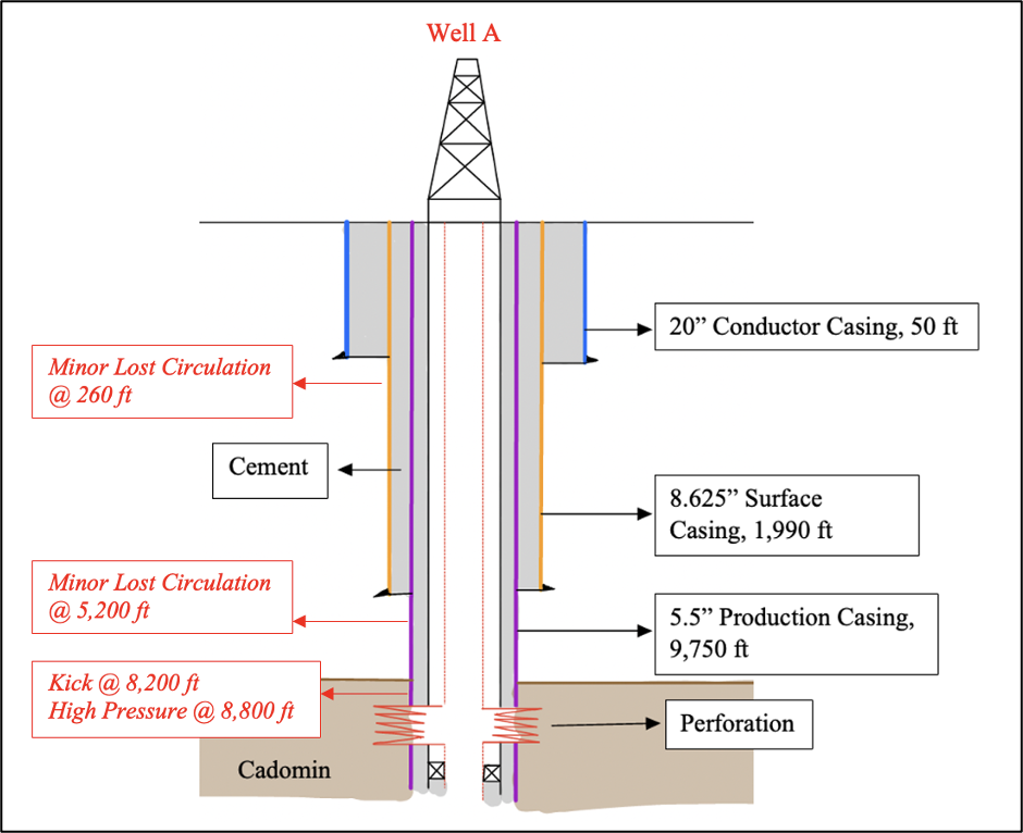
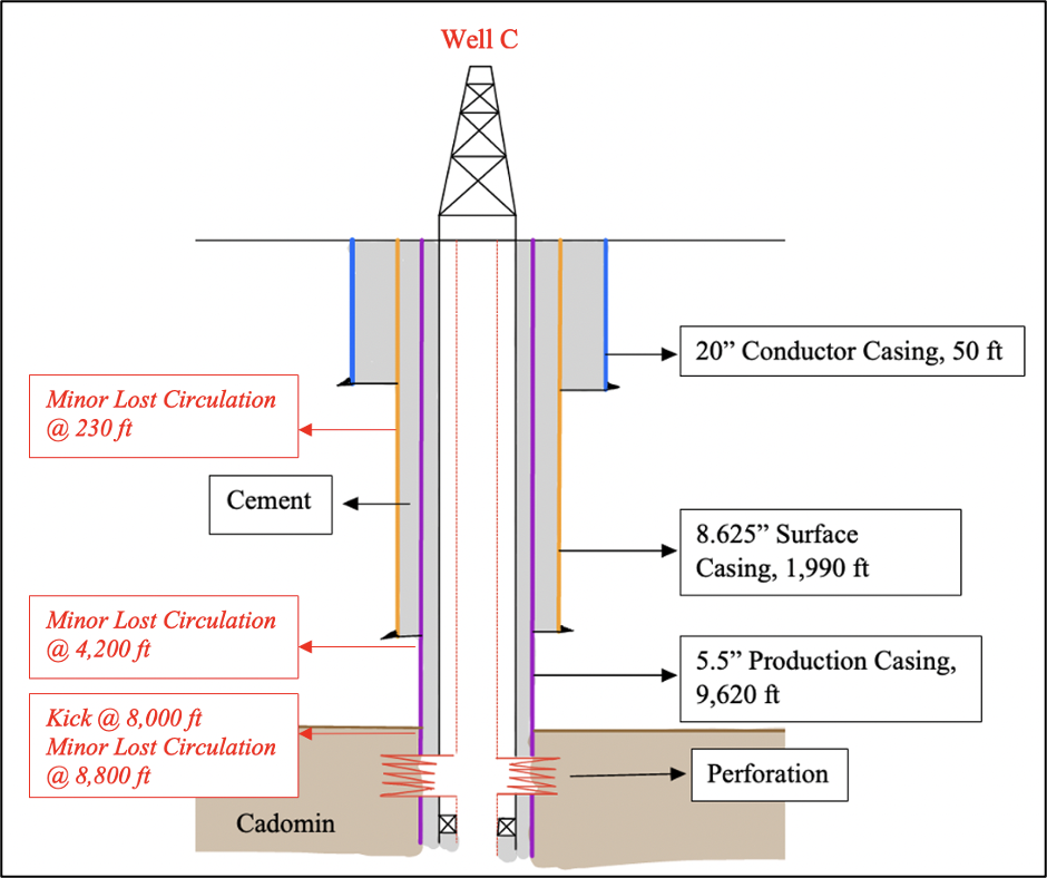
As part of the drilling and completion program for the vertical wells, underbalanced perforation completion is proposed. Perforations in well A and well C will be completed using a Tubing-Conveyed-Perforating (TCP) Gun. TCP allows perforations to be completed in a single trip and allows the well operator to perform a flow test immediately after perforation. It also has higher shot density than other perforation system such as through-tubing. Perforation will be completed at the depth of 9,700 ft (TVD) for well A and at 9,620 ft (TVD) for well C. Both of the depths are at the top of the pay zones, and aim to provide an easy access for induced production to flow through the production well. Dynamic underbalanced perforation is a perforation optimization scheme where pressure in the wellbore is lower than the formation pressure. The pressure differential is the main driver in creating undamaged perforations in order to optimize well productivity. It is suggested that higher underbalanced pressures are needed to obtain cleaner perforations.
6. MODELLING AND SIMULATION
Modeling the Cadomin formation in Township 66 on CMG allows us to ultimately forecast the production rates for the proposed infill wells. Reservoir Initialization is a critical step in the Simulation process as it establishes the dimension/orientation, property distributions, and original gas in place (OGIP) in the modelled reservoir. From the initialization process, OGIP was able to be determined from the simulation with CMG’s IMEX module. The OGIP values calculated for the entire township was 374.78 BSCF.
After the initialization process is completed, history matching can be done to calibrate the model to the actual production data obtained in the field. Gas rates from existing wells is imported from geoSCOUT, starting from initial production dates through July 2020. With calibration in place, infill wells (Wells A, B, C and D as proposed in the Drilling and Completions section) can be placed into the model to estimate the pressure and production trend, which will later be used in the economic analysis.
More details can be in seen in the sub-sections below.
6.1 Initialization
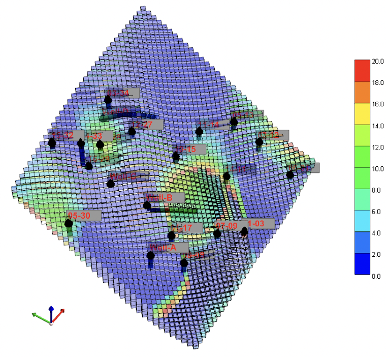
A township consists of 6 x 6 sections, and each section is further divided into 4 x 4 legal subdivisions (LSDs). Earlier versions of the model used a 24 x 24 grid in the i and j direction, each block in the model would represent one legal subdivision. However, this model was deemed to be too coarse, and a 48 x 48 model was developed to further refine the grid. In regards to the z direction, careful observation of the lithology from log interpretations showed four distinct layers within the Cadomin formation. Therefore, the dimensions of the model are 48 x 48 x 4 with a total of 9216 blocks.
An additional consideration made was to make the grid orthogonal. A 45° tilt was added to the grid in order to align to the direction of the maximum horizontal stress. In order to fit a 48 x 48 square in an orthogonal grid, a larger 72 x 72 grid was made and the outside blocks were simply nulled out. A 3D view of the model can also be seen in below.
In order to get the property distribution of parameters such as porosity, permeability, water saturation and pay thickness a surface mapping software known as Surfer was utilized. First, the aforementioned properties of each well in the township were obtained from geoSCOUT and were presented as data points to Surfer. Surfer essentially interprets data points and interpolates contour maps for each property. The datasets generated were then exported to the Builder module in CMG.
Data from PVT studies (pressures, formation factors, densities), and core analysis (relative permeabilities, water saturations, rock compressibility) were added to complete the Components, Rock-Fluid, and Initial Conditions sections. Perforations were set in each of the Cadomin wells and production was initialized based on the actual first production dates found on geoSCOUT.
6.2 History Matching
Because some wells produce from multiple formations at the same time, a correction factor based on the length of perforations in each formation is implemented to properly estimate the gas produced from the Cadomin formation alone.
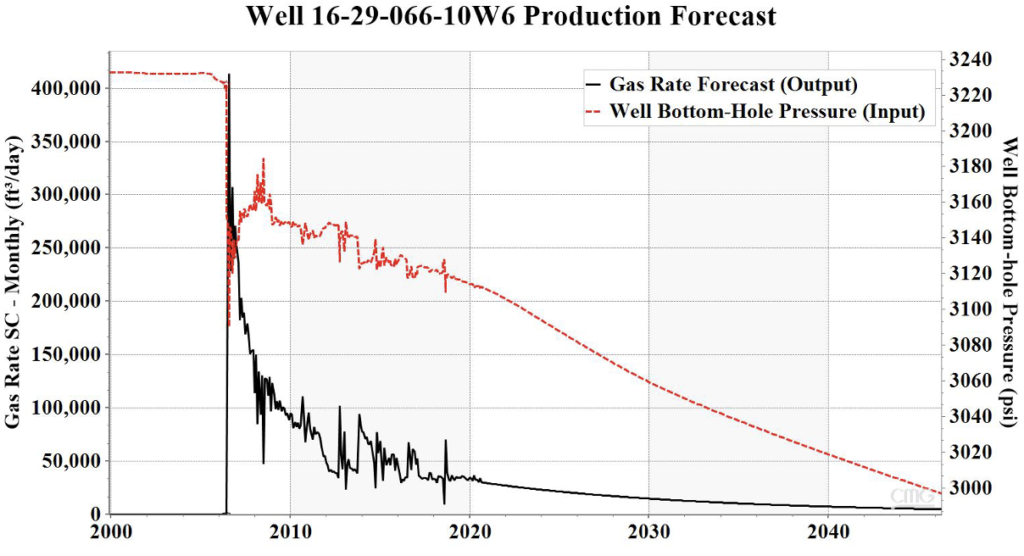
Based on the hydraulic fractures and the reservoir properties around the well, IMEX calculates the pressure drop required to sustain the production rates specified. These bottom-hole pressure trends are plotted on Excel and decline curves are generated to forecast the BHP over the next 25 years.
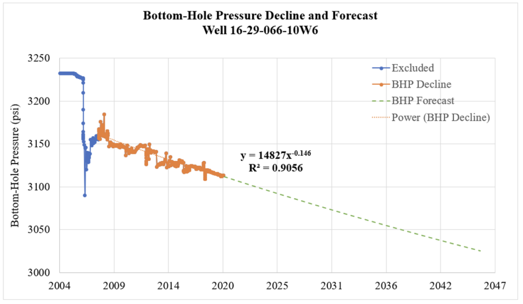
The extrapolated BHP decline curves are then exported back to CMG and the simulator uses these pressure values to predict the gas rates until May 2046.
6.3 Infill Wells (A, B, C, D)
Infill wells are then added to the model. Their placement depends on the rock properties distribution in the township with porosity, permeability, pay thickness and gas saturations taken into consideration. Also, nearby wells performance, proximity to gas facilities and access to pipelines need to be accounted for.
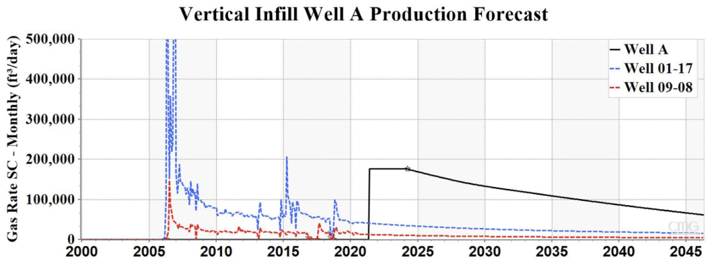
Desired production rates are estimated based on nearby existing wells performance and the capacity of the field facilities. Vertical well A’s initial production was designed at 175,000 SCF/day for example based on wells 01-17 and 09-08 historical gas rates.
7. PRODUCTION FORECASTING
After building the reservoir model and implementing the infill wells, production forecasting can be made for those wells based on the model’s property distribution and fracture geometry design. Once a production forecast has been made for the initial fracture design (the base case), changes to the infill wells can be included to investigate how the production is impacted by the fracture geometry. The two main fracture properties that were studied on are fracture stage spacing and fracture conductivity.
More details can be in seen in the sub-sections below.
7.1 Base Case
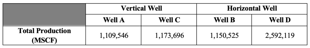
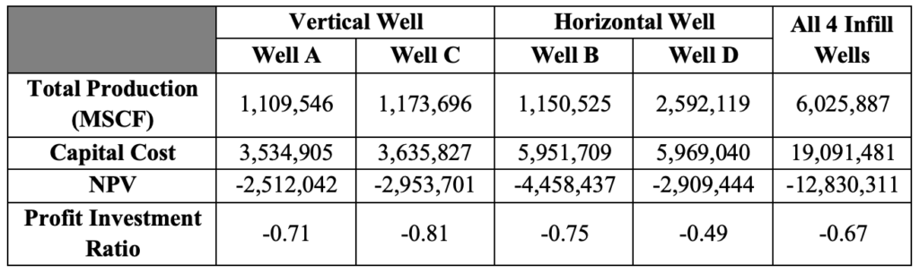
The base case for the four infill wells (2 horizontal and 2 vertical) was run with the same initial fracture geometry design. The production forecasted was based on the bottom-hole pressure distribution of the nearby wells for each infill well. The total production forecasted (for 25 years since 2021) can be seen below:
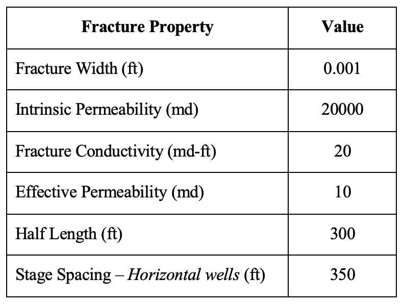
And the initial fracture design are with the parameters shown here:
7.2 Development Strategies
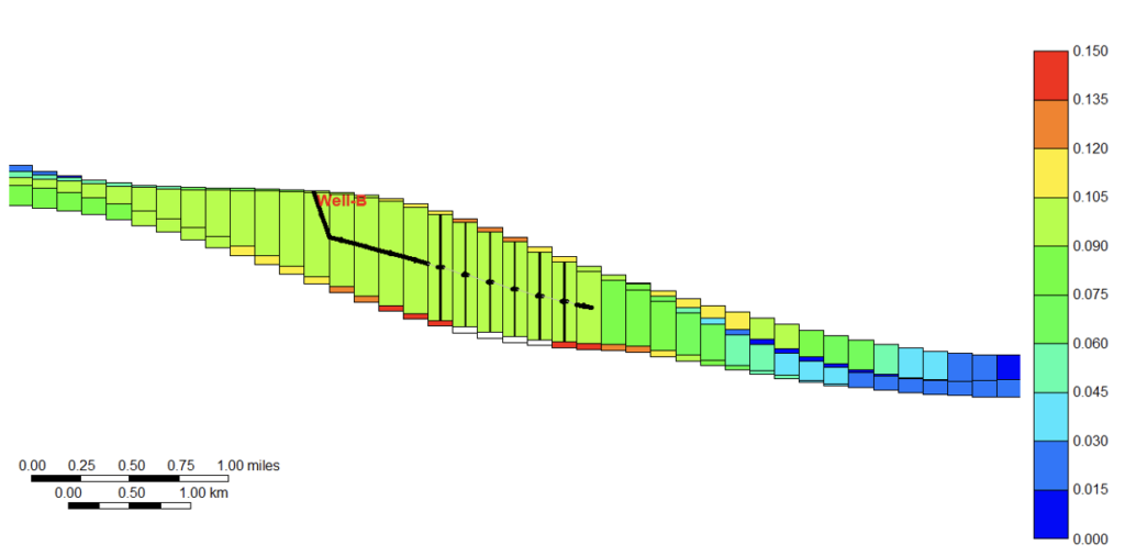
The development strategies were simulated using Well B as a standalone model. This reduces the complexity of the analysis especially with external factors that may affect the well B production such as production draw from nearby wells. The analysis below provides a focused discussion on the strategies mentioned.
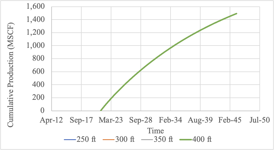
- Varying Fracturing Stage Spacing: It can be observed that changing the fracture spacing, whether it is decreased or increased, did not affect the cumulative production at any point. This implies production is not affected by fracture spacing and number of frack stages.
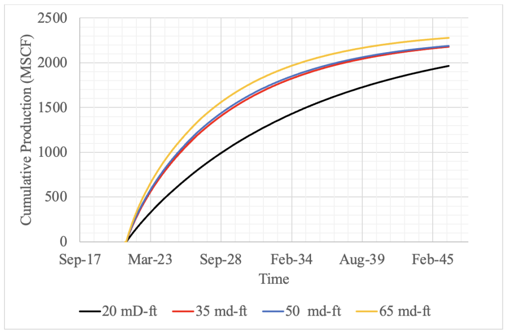
- Varying Intrinsic Permeability (Fracture Conductivity): The results shown here shows increasing fracture conductivity would increase overall production. However, an interesting trend that can be observed is that with an incremental increase of 15 md-ft for each trial, the marginal increase in cumulative production is not constant. This could be due to many factors that are related to the pressure propagation of the fracture and the geomechanical regime of where the fractures were induced.
8. PROCESSING FACILITIES
In the steps from gas produced at the well to gas within a transmission pipeline, gas processing is critical to ensuring the quality and specifications of the gas. Gas processing is the separation of the various components within the produced gas. Primary gas processing occurs in a gas processing plant where various unit operations are applied to separate the components found in natural gas. There is also a field gas processing step, where gas produced from the well is crudely separated before it is sent to the gas facility for further separation. The composition of the gas entering a pipeline must meet the specifications set by the pipeline operator. This usually includes certain restrictions on the amount of hydrogen sulfide and carbon dioxide, and minimum acceptable levels of methane or ethane to meet a given heating value. The process of purifying the gas allows the operator to know exactly what the composition of the gas is before it enters the transmission pipeline for transport across larger distances. At this point, the gas can be sold to consumers who require certain compositions of gas.
Gas hydrates are ice-like-solids that form as a result of a water and methane mixture in low temperatures (~32°F depending on pressure) and high pressures. The higher the pressure, the higher temperature at which gas hydrates may form. The plugging of the pipeline ultimately reduces the diameter and reduces efficiency. It may be as severe a pipeline burst from the build-up of pressure from the choke point caused from gas hydrates. Removal of water via condensation or glycol dehydration acts as one of the major ways to control and prevent the formation of gas hydrates.
More details can be in seen in the sub-sections below. Or for more details about the design, please join us at our Zoom Meeting room to learn more.
8.1 Field Gas
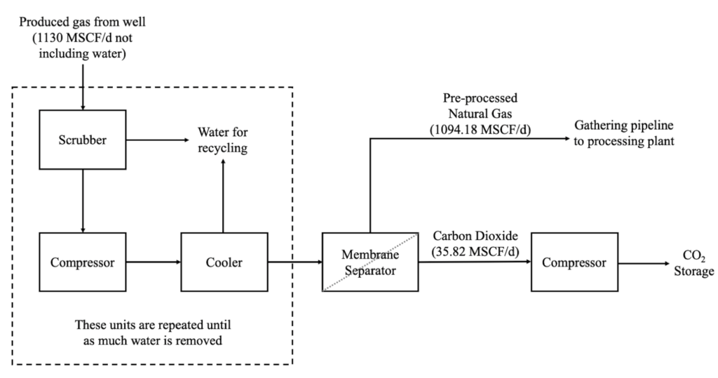
Field processing is required to prevent downstream equipment damage and downtime. Pre-treating the gas removes any potentially freezable components that may cause pipeline bursts from a build of up pressure if the solids block the flow path of gas.
CO2 (acid gas) removal with membrane separation is necessary to ensure that the quality of the final gas is not compromised and to also meet pipeline specifications. Current Canadian pipeline specifications require that the CO2 concentration must be within 2% by volume. The average produced gas composition from the Cadomin yields a CO2 concentration of 3.17%. The removal process is carried out with a Deca-Dodecasil 3 Rhombohedral (DDR) zeolite membrane. The DDR membrane is highly selective to carbon dioxide over more conventional polymeric membranes, and methane losses are minimized.
Compressor units are installed to aid in the production from gas wells. This is especially useful for gas wells that are almost abandoned or nearing the end of their producing life. Multi-stage compression helps balance the load between each stage to prevent overloading the compressor. Overloading the compressor can lead to a reduction in compressor efficiency, and an increase in energy consumption. Intercoolers (shell-tube heat exchangers) are provided between stages to help remove the heat of compression from the gas and reduces the work needed to compress the gas for the next stage.
8.2 Gas Processing Plant
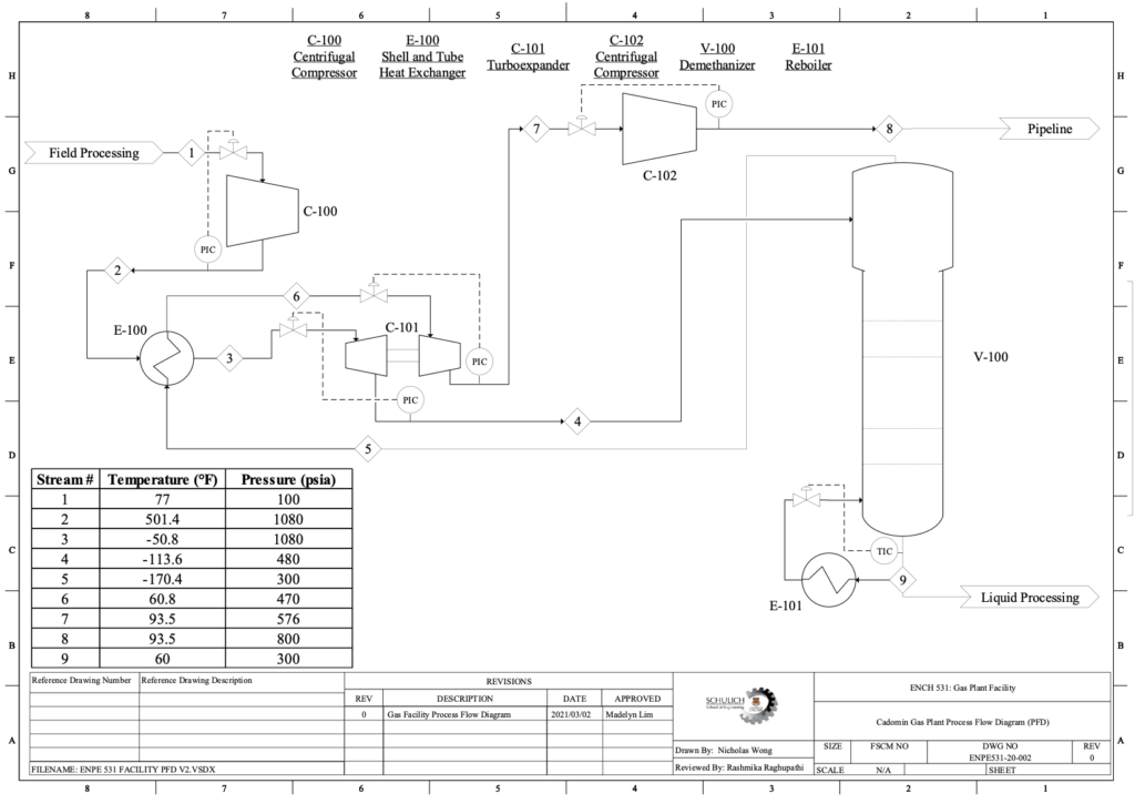
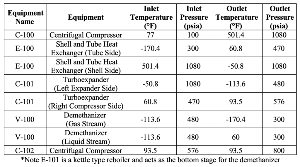
As the gas enters the processing facility from the field processing, it is first compressed to the appropriate pressure required downstream in the hydrocarbon separation unit with a centrifugal compressor (C-100 and C-102), either a continuous-flow compressors or turbomachines. The gas stream enters compressor C-100 at a temperature of 77°F and 100 psia. It then undergoes a four-stage compression where the discharge stream is at a temperature of 501.44°F and 1080 psia. C-100 and C-102 were assumed to operate at an efficiency of 75%.
After the compression step, the gas is cooled down by a heat exchanger (E-100) to bring it to a temperature where any remaining water present in the gas can condense. Any remaining liquid that condenses during this process is removed from the gas as part of the final water removal step done to ensure there is no possibility of water for the following cryogenic processes. The heat exchanger will have counter-current flow arrangements to ensure that there is a uniform temperature difference throughout the heat exchanger, thereby minimizing thermal stresses. The area available for heat transfer in the heat exchanger is 2166 ft2.
After the cooling/condensation step, the gas temperature would have been lowered through turboexpansion to allow for the water to condense, but this also prepares the gas to be further cooled before the hydrocarbon separator. The turboexpander (C-101) works as a combined expander and compressor unit, where the gas that flows in on the compressor side is separate from the gas that flows in on the expander side. These two piece of equipment are connected with a shared shaft in the middle, thus energy generated in the expansion process is used to compress gas on the compressor side. This process that occurs within the turboexpander is isenthalpic, or an ideally reversible and adiabatic operation. Due to this, the heat removal from the expansion process due to the pressure drop is at its maximum amount. The temperature necessary for this separation is approximately -148°F (-100°C). This lies between the boiling point temperatures of ethane, -128°F (-89°C) and methane, -260°F (-162°C) which allows the ethane to condense into a liquid while the methane remains a gas. To determine the wheel diameter of the turboexpander, a specific speed of 75 is assumed with a design efficiency of 70%
The cooled feed leads into a demethanizer column (V-100) that results in a very pure stream of methane gas from the top of the column while the remaining hydrocarbon components are removed. The demethanizer works by exploiting the temperature difference in the boiling points of all of the components within the gas. By bringing the mixture to temperatures between the boiling points, certain components will condense out and separate from the mixture. There are approximately 18-26 trays within the demethanizer column to section off areas for the gas to condense and allow for proper flow of fluids through the entire column. The size of the top column is significantly larger to accommodate for the amount of the vapour feed within the tower. It acts partially as a flash drum for the entering fluid. there is a reboiler at the bottom to further purify the bottoms liquids. This bottom reboiler (E-101) acts as the final equilibrium stage at for the column. The overall column efficiency is estimated to be 77% will be used for the demethanizer as the overall efficiency of the separation for the methane from the other components. The remaining natural liquid gases of ethane, propane, butane and other longer chained hydrocarbons are further processed for liquid processing for further separation between each component or can be sold as a mixture of these liquid. The purified methane stream leaving from the demethanizer is 97 mol% methane, 1.5 mol% ethane, 1.0 mol% nitrogen, 0.2 mol% propane and with the remaining consisting of small trace amounts of hydrogen, helium, butane and other longer chained hydrocarbons.
9. PROCESS SAFETY
The identification, evaluation of hazards, and the development of appropriate strategies to mitigate and manage residual risks is a fundamental requirement for any industrial process. With the health and safety of the process and operators as top priorities, this analysis utilizes risk management tools and methodologies that are in accordance with the APEGA. The assessment for multiple health, safety, environmental, and financial risks using a HAZOP methodology is to be completed to minimize project risks to as low as possible. From this assessment, the enhanced design would be environmentally and socially sustainable. A HAZOP is to be completed on the P&ID created for the shell-and-tube heat exchanger, E-100. An initial risk rating was assigned to each risk scenario based on the likelihood of it occurring and its consequence, with consideration for the mitigating measures and safeguards indicated on the P&ID.
More details can be in seen in the sub-sections below.
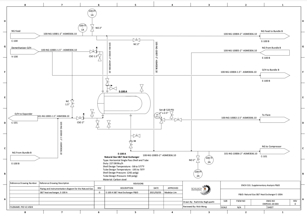
9.1 Hazard and Operability Study (HAZOP)
Through the HAZOP, control elements are incorporated into the design to minimize any potential risks. The complete HAZOP analysis, mitigating measures, and the full list of recommendation/action items are included in this section. The cause, consequence, and risk rating are initially completed under the assumption that no safeguards are in place. Recommendations for risk mitigation and reduction were then made for hazards that have an unacceptable or conditionally tolerable risk rating, and the residual risk was studied again. In some scenarios where the risk level was acceptable and a strategy was devised to further reduce it, a recommendation was still made.
Some examples of the control and safety elements taken into consideration are:
- A bypass line on both the shell and tube sides on E-100 A to allow for a bypass route to E-100 B in the event of equipment upsets.
- Block and vent valves on the inlets and outlets of E-100 A to allow operators to isolate the heat exchangers and prove zero energy for maintenance purposes.
- A parallel bundle, E-100B, will be used in the event that E-100A is decommissioned for maintenance/ cleaning purposes so as to ensure continuous operation of the gas plant.
- A check valve is also present on the shell inlet from C-100 and the tube outlet to C-102 to prevent backflow into the heat exchanger lines in the event that the compressors surge.
- Pressure safety valve (PSV) was designed to protect the tubes of the heat exchanger in the event that the operator closes the cold tube isolation valves and leaves the hot process side running.
The full HAZOP worksheet can be found here:
10. ECONOMICS AND SENSITIVITY ANALYSIS
The economic analysis was conducted based on the prediction that the gas wells drilled will produce for over 25 years, from 2021 to 2045 based on the production forecasted in the reservoir simulation. This time period was selected as it captures the period to determine if a well will be profitable in the long term. If the well is ran long enough to the point where the operating costs outweigh the profit from the produced gas, then it is clear the well should stop production before this point. The gas price was forecasted for future years fitting a polynomial curve to GLJ gas price forecasts, measured per gigajoule.
From the economic analysis, all of the wells do not produce a profit and have a negative NPV after the 25 year period. This is due to the low gas prices and gas rate produced from the wells that did not outweigh the initial capital cost.
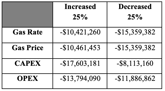
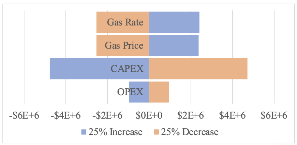
A sensitivity analysis demonstrates the variability of a project to economic conditions and how the economic indicators would change. The proposed four well development will be used for this sensitivity analysis. The calculated NPV after 25 years will be used as the economic indicator, with the base case NPV to be determined as -$12.83 million. The analysis concluded that the capital cost has the largest impact on the NPV, followed by the gas rate and gas price, and that a 25% increase or decrease of any of the variables such as CAPEX and OPEX was not enough to result in a profit.
A probability tree determines the statistical risk associated with each decision. In this project, it will be used to breakdown the probability for a successful well. The cost for drilling the wells is fixed and then the probability for gaining a profit based on each route determines the final revenue for the project. The analysis was carried out on vertical wells only, and is split into two sections – one for Cadomin-only wells, and one for commingled wells. Based on the results, it is recommended to complete vertical wells drilled as commingled, rather than targeting Cadomin only.
More details can be in seen in the sub-sections below.
10.1 Economics Analysis
Net present value (NPV) is used as the main indicator to determine if the project is economical or not. In the case that the NPV is positive, the company is expected to return an income. If the NPV is negative, the project is no economical and will lose money. Other economic indicators such as the payout period, internal rate of return and the profit investment ratio can be considered. When determining the NPV, the operating cost, capital cost, taxes and royalties were considered, along with a 10% discount rate, which is commonly used for oil and gas companies.
The gross revenue can then be determined by multiplying the produced gas from the production method, by the price of gas and the energy conversion. The tax rate that is applied to projects in Alberta is based on both a provincial and federal tax rate. The provincial tax rate is set to 8% as of July 2020, while the federal tax rate is 15%, for a total tax rate of 23% (Alberta Government, n.d.). This represents a total of 23% of taxes removed from the gross revenue. Using the Modernized Royalty Framework provided from the Government of Alberta, the royalty percentage rate can be calculated, which ranges from 5% to 36% depending on the revenue of the project.
Capital cost is mainly the drilling cost, which contains a detailed breakdown of the individual costs for planning, construction, drilling and completions. Operating costs were estimated based on fixed and variable costs. Fixed costs are costs that remain the same and do not vary based on any other variable. This includes costs such as the land lease cost per section. Variable costs change according to a variable that changes during production.
The results from the analysis are summarized in the table below:
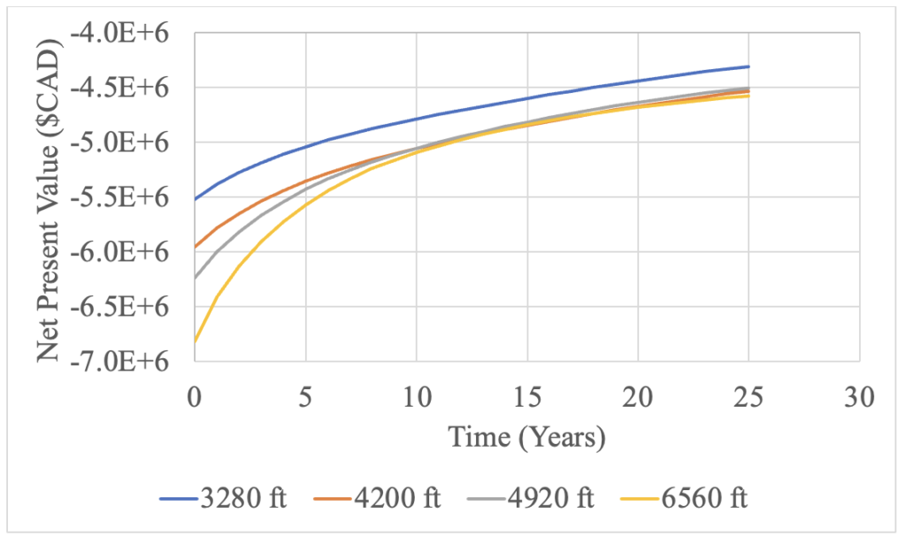
10.1.1 Optimization
The economic optimization of the fracture spacing is performed on a simulated test well within the township. This is in the same location with the same properties as well B, a horizontal well. This standalone well will have the horizontal lateral length varied and the optimum spacing can be determined from the trials. The reference case is a lateral length of 4200 ft with a total of 12 fracture stages. As the lateral length is varied, the total amount of fracture stages changes as well as the initial capital cost. A constant stage spacing of 350 ft is used for this optimization. For the optimization horizontal lateral lengths of 3,280 ft, 4,200 ft, 4,920 ft and 6,560 ft were used each with 9, 12, 14 and 18 fracturing stages respectively. From the optimization, the best option is the lateral length of 3,280 ft and 9 stages. In the case that the wells were economical and producing a profit this analysis may reach a different conclusion.
10.2 Sensitivity Analysis
As for the sensitivity analysis, variables such as the natural gas cost, produced gas, capital expense and operating expense will be varied to analyze the NPV sensitivity. A percentage of plus or minus 25% for each of these variables is used. Each variable will be altered and the resulting NPV is recorded (shown in the table below). A combination of increased gas rate, increased gas price and lowered capital costs would result in a higher NPV. Due to the fluctuations experienced in the energy industry unexpected drops or increases in demand often occur and the outlook of the gas price may change greatly in future years.
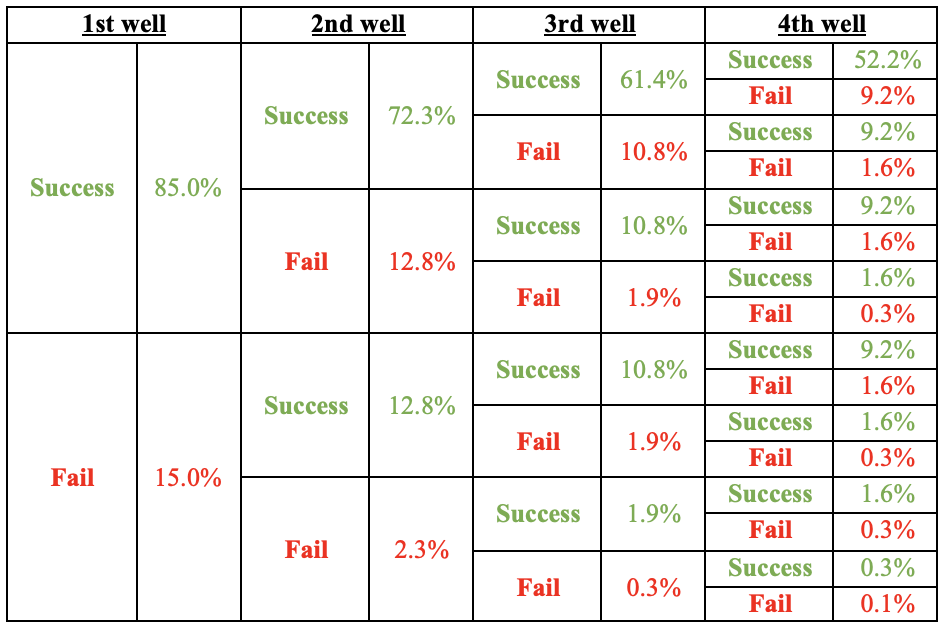
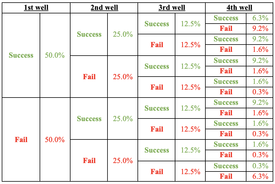
With regards to the probability tree, the analysis will be performed on vertical wells only, as there is only historical data in the township for vertical wells. A successful well is defined as a well that is producing gas as predicted, while a failed well is one that does not produce gas at all. A probability for each well is determined from existing historical data on active versus abandoned wells. The final probability for the resulting NPV gives insight to a company as to the risk associated with the project and the chances they have to generate the target revenue. The analysis will be split between commingled wells and Cadomin only wells. There are 5 scenarios that can result, all 4 wells fail, all 4 wells are successful, one, two or three wells are successful with the others failing. Each of these scenarios will have their own respective probability and will follow a binomial probability distribution.
For commingled wells, the probability for a successful commingled well was determined as 85%, and a 15% failure rate for the well to not produce gas at all. The success rate for all 4 wells drilled to be successful is 52.2%, which results in a NPV of -$10.05 million. As encountered in the previous analysis, the NPV is negative, indicating that this project does not return a profit at the current gas rate and economic market.
For Cadomin-only wells, with only 3 active existing wells, this resulted in a 50% chance for both a successful and failed well. The highest probability lies at 2 successful wells with 37.5%, followed by 1 or 3 wells at 25%.
The probability tree constructed for each analysis is shown below:
Partners and Mentors


Photo Gallery
LOG INTERPRETATIONS
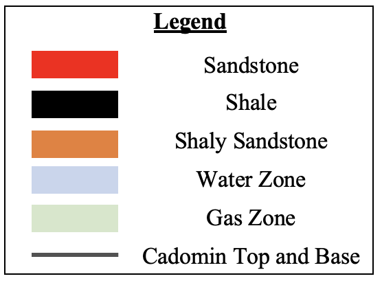
Legend for log interpretation figures. 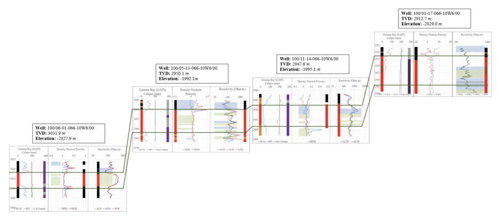
Log interpretations. 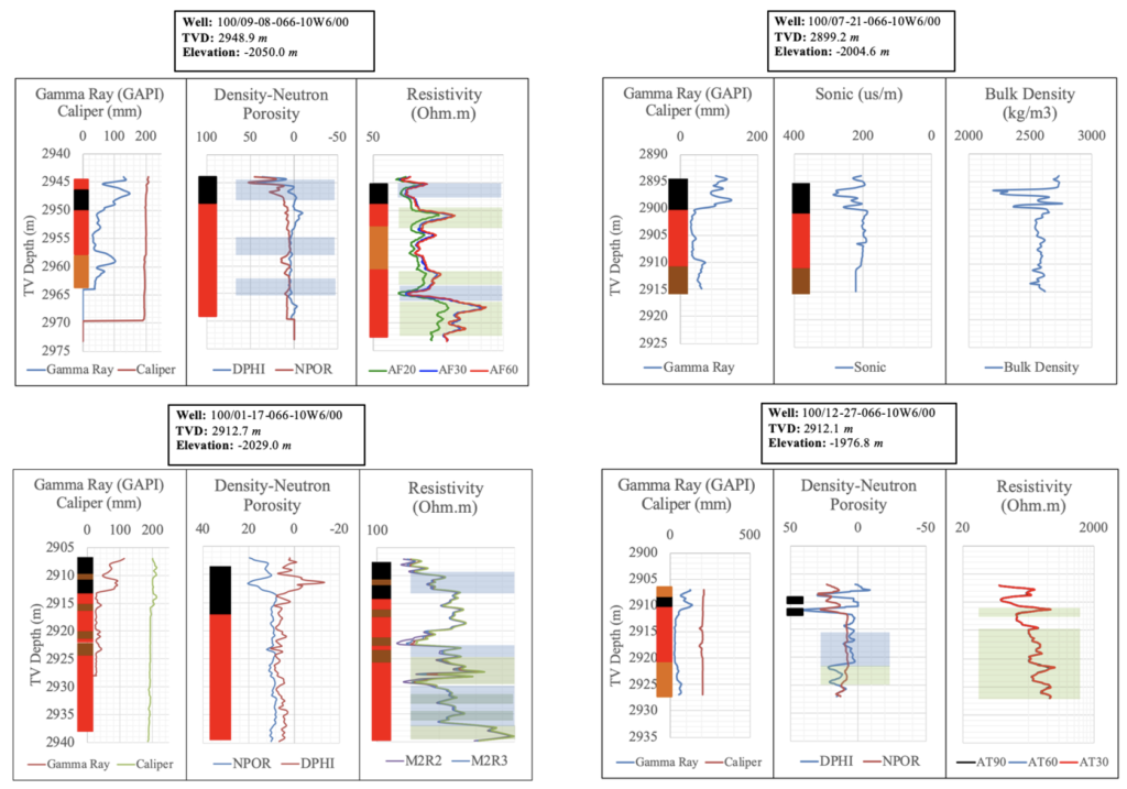
Log interpretations (cont’). 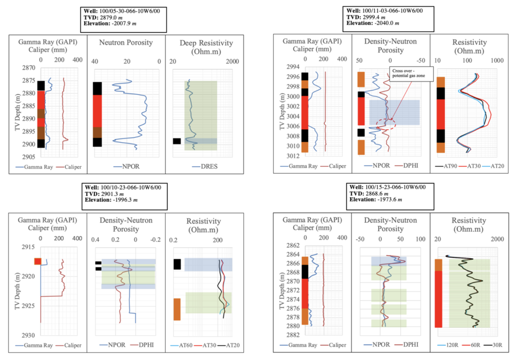
Log interpretations (cont’).
MAPS
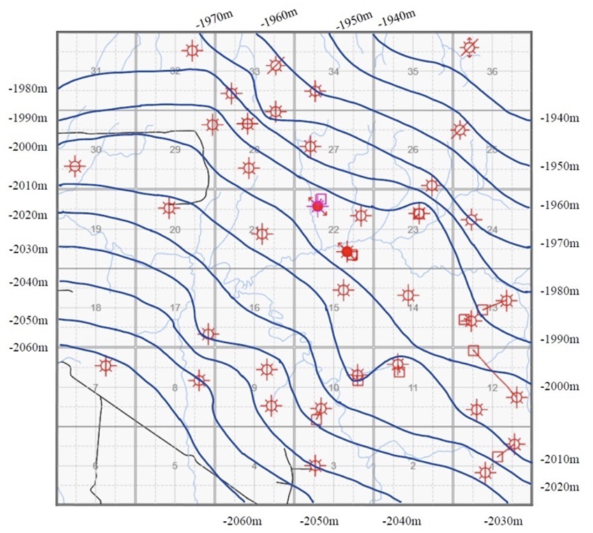
Cadomin Top. 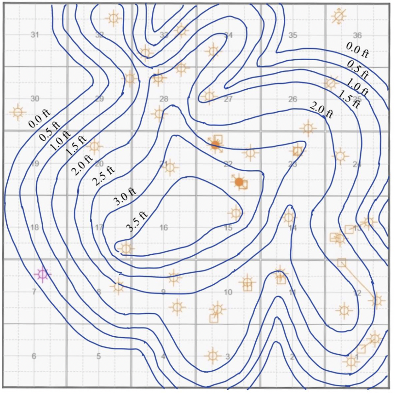
Producible Zone Thickness. 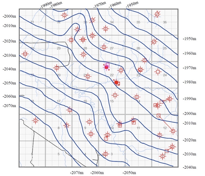
Cadomin Bottom.
