Project Category: Petroleum
We will be in the Zoom meeting from 9:30 am – 1:30 pm on April 5th, 2022.
Click the link above to come and chat with us after you have watched our presentation!
About Our Project
The story begins in 1979 about 60km west of Drayton Valley with the first producing well in the Basal Belly River formation. Log and core analysis showed that this is a titled reservoir, deeper in the west and shallower in the east, with a shale layer running through the middle of the pay zone. The reservoir was initially owned and operated by TORC in the west and Whitecap in the east, until recently when Whitecap acquired the whole pool. Due to the different operating strategies throughout the life of the pool, the waterflood management differed on either side and potentially resulted in pockets of trapped recoverable oil. Our objective was to investigate the current status of the pool and provide economically feasible development strategies to optimize the waterflood and provide further oil recovery.
The Problem: High water cuts and low production rates.
The Objective: Optimize the waterflood to increase production rates in an economically feasible way.
The Solution: Let’s find out!
Meet The Team

Aleisha Raman-Nair
Chemical Engineering with
Minor in Petroleum

Alexander Connick
Chemical Engineering with
Minor in Petroleum

Andres Caceres-Soto
Chemical Engineering with
Minor in Petroleum

Matthew Cochrane
Chemical Engineering with
Minor in Petroleum and
Entrepreneurship & Enterprise

Sydney Usselman
Chemical Engineering with
Minor in Petroleum
Details About Our Project
Understanding The Reservoir
Geology
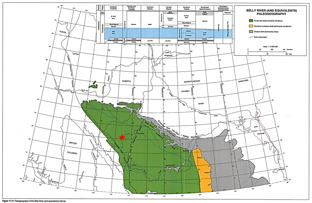
The sands of the Belly River Formation were deposited in the Campanian age of the Upper Cretaceous Epoch. The Belly River Formation is within the Western Canada Sedimentary Basin which ranges from Central Alberta to Southeast Saskatchewan [1] as shown by the green area in the image below. Much of the Belly River Formation is comprised of sandstone-rich channels interspersed with mudstone-rich floodplain deposits [2]. The Basal Belly River formation is primarily very fine to medium grain sandstone, poorly to well sorted, the grains have low sphericity, and are loosely packed with calcite cement [3]. Non-continuous layers of shale between sand bodies as well as clay-rich calcite cemented rocks that form lateral permeability barriers can be found in the formation [3]. There is an obvious coal seam beneath the main producing sand body which indicates the continental nature of the sand above, and the marine sand and shale beneath. Core data confirmed the presence of other rock types and minerals such as pyrite, conglomerate, dolomite, calcite/carbonate, and argillite, with most of the formation being fine sandstone with shaly laminations present.
The source of hydrocarbons for the Belly River Formation comes from the Colorado Group Shales, more specifically the Second White Speckled Shale [5]. The Basal Belly River Q Pool has a stratigraphic trap made by the underlying strata consisting of low permeability shale of the Lea Park Formation and the overlying strata that is also a lower permeability shale. The over and underlying shales provide a seal for the hydrocarbons of this pool.
Reservoir Properties
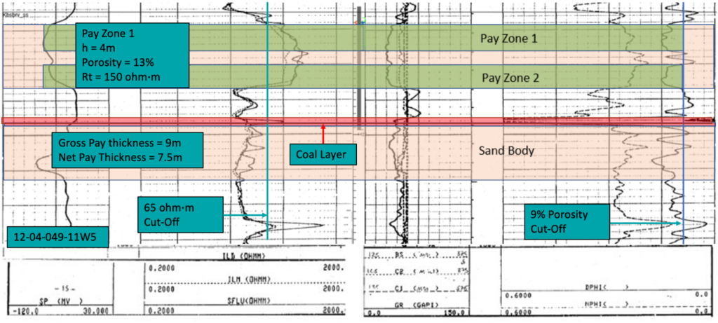
Log and core analysis were critical to effectively determine the reservoir architecture, pay zones, and obtain reservoir properties such as porosity, permeability, and water saturation. The analysis provided average east and west properties as summarized in the table below.
| Property | West | East |
|---|---|---|
| Pay Thickness (m) | 5.3 | 3.8 |
| Porosity (%) | 12.7 | 11.3 |
| Permeability (mD) | 68 | 9 |
| Water Saturation (%) | 29 | 30 |
The detailed data obtained for each well was utilized to create maps which assisted in calculating the volumetric original oil in place as 4.34 million m3 of oil, which is compared to other sources below.
Simulation OOIP = 4.27E6m3 (-1.6%)
Whitecap OOIP = 4.39E6m3 (+1.2%)
The reservoir was found to be initially undersaturated with an initial pressure of 10750 kPa and a bubble point of 9270 kPa. The oil produced is quite light with a density of 815 kg/m3.
Following the material balance analysis, it was determined that there is an active aquifer present in the western-most edge of the pool which explained the behaviour of the production history pre-injection. The aquifer presented many uncertainties since there was minimal tangible evidence (no log data) to confirm the location and extent of the aquifer. However, all analysis and investigation pointed toward an aquifer being present and hence it was necessary to include it.
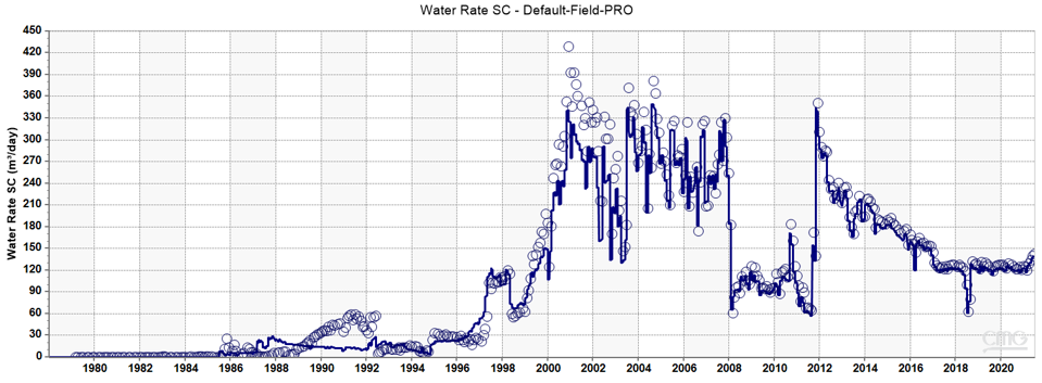
Production History
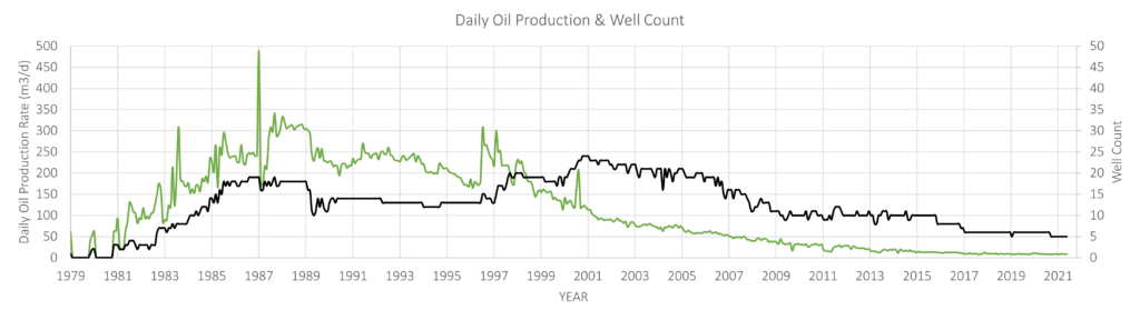
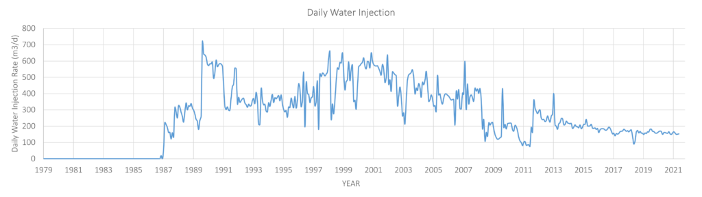
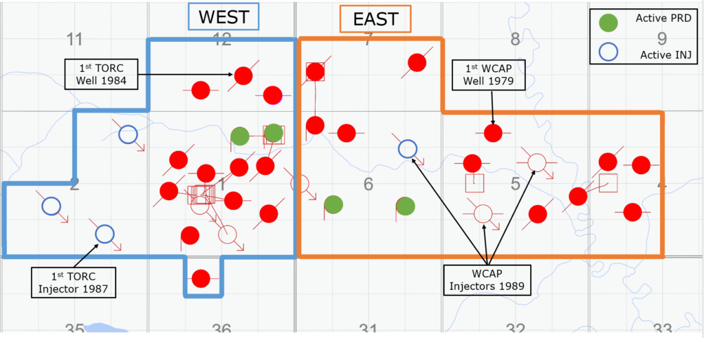
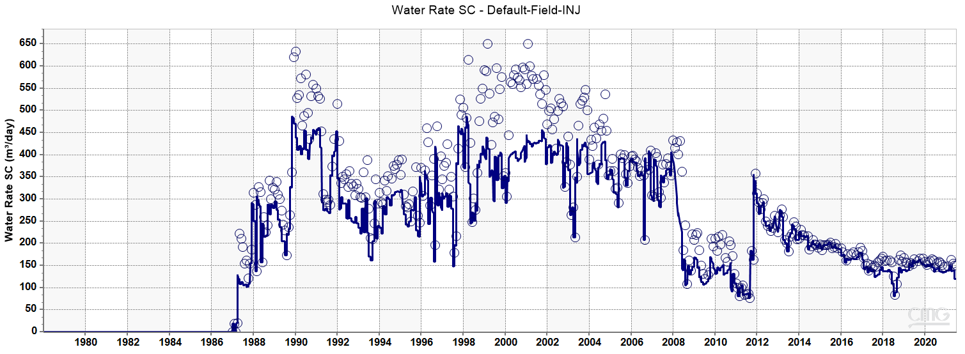
Oil production began in 1979 in the eastern end of the pool and in the years following, new wells were brought on totalling 11 Whitecap producing wells by 1984. TORC drilled its first well in 1984 in the west, which had a very high initial water cut due to water influx from an aquifer. Since the aquifer influx caused high water cuts, TORC began swapping the producers into injectors in 1987 and so began the waterflood.
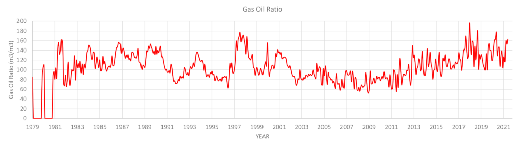
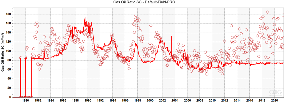
The water injection only seemed to support the west side of the reservoir, as the east drops below bubble point pressure soon after injection begins. In response to the east dropping under bubble point, Whitecap swapped three lower producing wells to injectors and began a waterflood in the east in 1989. Following this water injection in the east, the reservoir pressure came back up and the GOR decreased as expected. From 1989 to 1994, both the east and west sides had established a waterflood which was successful in producing at a relatively stable rate until the end of 1994, when production started to decline due to water breakthrough.
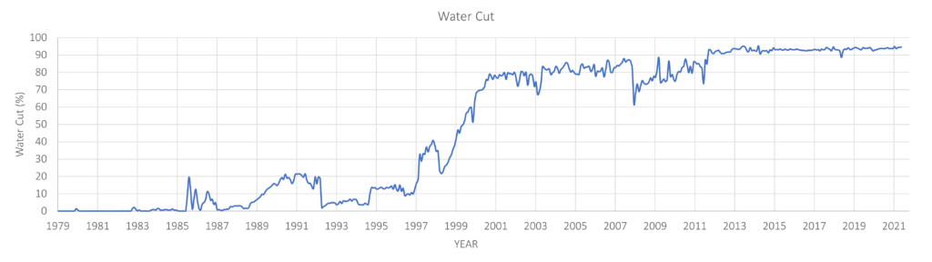
Following breakthrough, high water cut wells were converted to injectors and an infill program and multiple well completions were executed in 1996. In 1997 the west side of the reservoir began to decrease in pressure and fall under bubble point as evident in the GOR spike, so injection rates were increased. After these actions, the oil production increased, and the water cut dropped temporarily. However, production began to continually decline, and the water cut reached nearly 80% by 2000. In 2008 there was a notable drop in water injection rates which was followed by an increase in GOR, and a sharper decline in production. By 2012 injection picked back up, but this seems to have a poor effect as production rate continued to decline and water cut increased to nearly 95%. After the water injection was increased again in 2012, the injection rate was slowly decreased as production continued to decline, GOR remained relatively constant, and wells were taken off as they reached abandonment rates.
Currently, the reservoir is producing 8.3m3/d at a 94.5% water cut. Cumulatively, this pool has produced 1.36E6m3 of oil, 1.76E6m3 of water, and 149.3E6m3 of gas, with 3.90E6m3 of water injected.
Waterflood Surveillance
Since the objective of the project is to optimize the waterflood of this pool, it was a pertinent step to perform a detailed waterflood analysis to gain insight into the connectivity and sweep efficiency within different areas of the pool. Results of the waterflood surveillance could then be used to highlight potential target locations for development strategies, as well as a basis to compare simulation results.
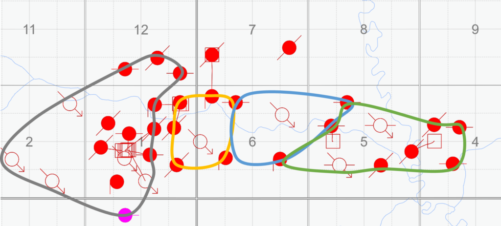
To begin the investigation, injector/producer patterns had to be selected. Patterns were chosen as shown in the figure below which was done after investigating production history and understanding connectivity within the pool.
The key plot used in the Waterflood Surveillance analysis was Recovery Factor vs Hydrocarbon Pore Volume Injected, which was created for each pattern. This plot shows the sweep efficiency comparison between individual patterns, overall reservoir performance, and the hypothetical maximum Buckley-Leverett estimate.
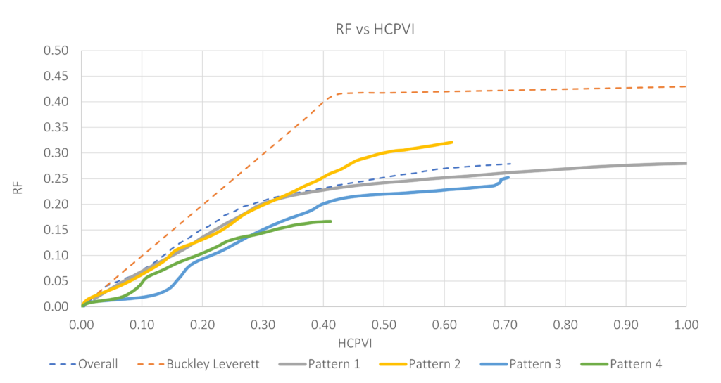
A detailed analysis of the results for each pattern is as follows:
Pattern 1 – Below average performance due to high injection rates required to increase and maintain reservoir pressure. It is predicted that the high injection rates may support the neighbouring high production rates in Pattern 2. It is suspected that this area is overall well-swept, with perhaps some oil remaining in the far southern and northern edges of the pattern. Not a prime target for further development.
Pattern 2 – Above average performance due to good connectivity within the pattern as exemplified by increased injection followed by improved production in each well. As aforementioned, the high production rates in this pattern may be supported in part by the high injection rates in Pattern 1. It is suspected that this area is overall well-swept and is not a prime target for further development.
Pattern 3 – Quite poor performance throughout which is suspected to be due to poor connectivity caused by the shale layer. The improved recovery near the end of the production is due to sustained production with greatly reduced rates, caused by only one operating and injecting well at the time. Additionally, there were instances within the study where the VRR was over 1, meaning higher injection than production. It is predicted this may have pushed oil into the northern and southern edges of the pool, making this area not well swept and a prime target for development.
Pattern 4 – Poorest performance which is suspected to be due to poor connectivity caused by the shale layer. After further investigation, it appears the lower producing sand layer is not perforated in some wells, which suggests the bottom layer is not well swept. The eastern edge of the pool is a prime target for further development.
Simulation as a Design Tool
Reservoir Simulation

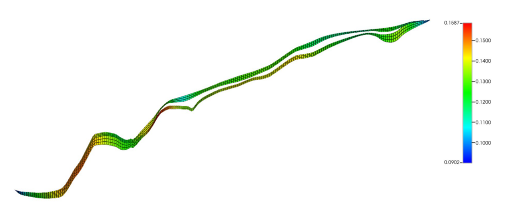
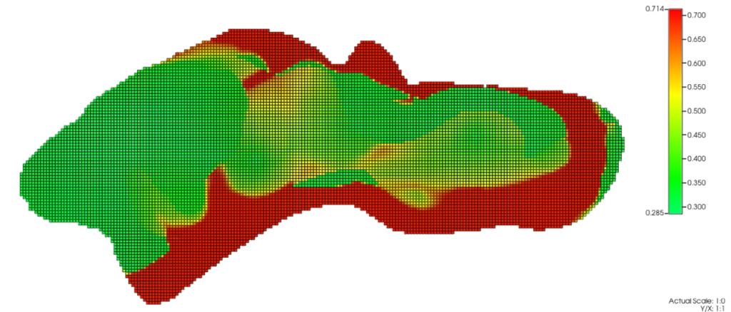
A reservoir simulation was built to assist in providing insight into how to proceed with the pool development. CMG Reservoir Simulation Software was used to model the reservoir using a Black Oil Model in IMEX as this reservoir follows the conventional black oil performance and is the most appropriate choice to model a waterflood. The reservoir was initialized using various maps to capture the structure and petrophysics, as well as raw data inputs such as PVT and Relative Permeability as obtained from Whitecap. The well trajectories, perforations, and historical production/injection data were also inputted. The image shown above highlights the tilted nature of the reservoir, with the lowest end in the west at 1530m up to the shallowest in the east at 1420m. The following image indicates the porosity distribution within the pool, showcasing the higher porosity zone in the west.
In order to adequately capture the structure of the reservoir and shale layer, three distinct maps were used, namely the top pay sand, a layer of shale, and the lower pay sand. These maps were attributed to different grid layers in order to effectively model the flow dynamics that the shale layer presents. A side view snapshot shown below shows the shale layer, which is assigned to null blocks and is discontinuous throughout the pool.
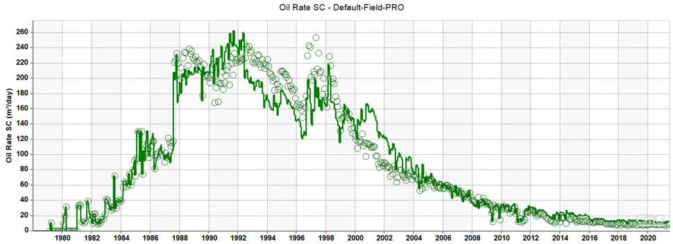
History Matching
With the simulation initialized, the simulation inputs were edited such that the historical data matched the simulation outputs. A good match between historical and simulation data is of high importance to ensure the model is accurate before utilizing it for development strategy investigation and forecasting. History matching is a highly iterative process and the best results thus far are shown here. Where the oil rates are not currently matching perfectly, specifically from 1992-1998, is most likely due to a lack of injection support in the model. Methods to better match injection rates are described in the following.
The high historical water rates in 1988-1992 are suspected to be due to the aquifer influx causing high water cuts occurring in the western edge of the pool at that time. Altering the aquifer parameters, such as decreasing the size and decreasing the permeability should slow down the water influx and shift the high water rates closer to the historical data.
The GOR and injection rates are parameters that require further investigation to obtain a better match. As mentioned previously, the injection rates are lower than the historical values which is perhaps causing the reduced oil production rates. It is suspected that the injection wells were in fact fractured due to high injection rates and pressures during early pool development, which is not currently being modelled within the simulation. Adding these fractures near the injectors is expected to improve the ability for the injection rates to meet the historical values by providing less resistance to flow with extra fractures in place.
The simulation history match will be investigated further, but nonetheless, the results provide further insight into the remaining pockets of oil that could be targeted. The remaining oil as predicted by the simulation is in a very similar location as what was predicted by the analytical Waterflood Surveillance. Since both the manual investigation and the simulation results tell the same story, the development strategies could be better justified to target the northern, eastern, and southern edges of the pool.
Our Solution To The Problem
Development Strategies
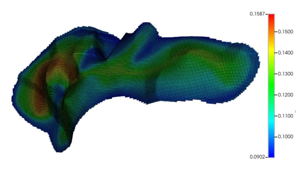
Based on the simulation results, it appears there are pockets of oil in the northern, eastern, and southern edges of the pool, which provides different options for further recovery. Since the current reservoir production rates are just over 8m3/d, we had to get creative to find economically feasible development strategies. Because drilling a new well is quite expensive, for our pool we also looked into “quick fixes” such as reperforating wells, restarting wells that were prematurely shut down, and using a different injection scheme with the existing wells. Locations were targeted using the “Oil Per Unit Area” figure partnered with the “Oil Saturation” figure as it provided more insight into the remaining volumes. The following development strategies were investigated:
- Turn well 07-01-049 back on.
- Turn well 01-12-049 back on.
- Reperforate well 06-04-049 into the lower pay sand.
- Drill horizontal well in the eastern edge of the pool, Section 4.
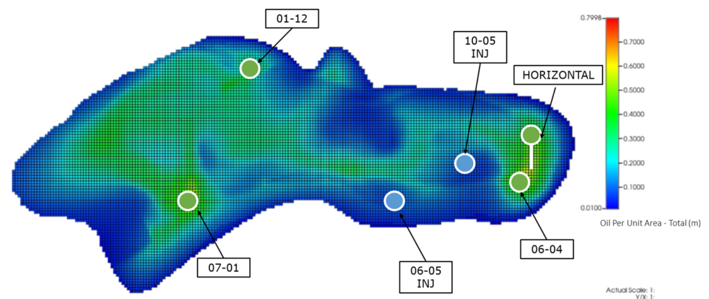
Along with these methods, turning on the injectors in 06-05-049 and 10-05-049 were also tested to try and find an optimal recovery scheme. Note that these strategies include leaving the current active wells operating, see About Our Project for the map indicating these wells.
The simulation was used to model and forecast each development strategy as shown here.
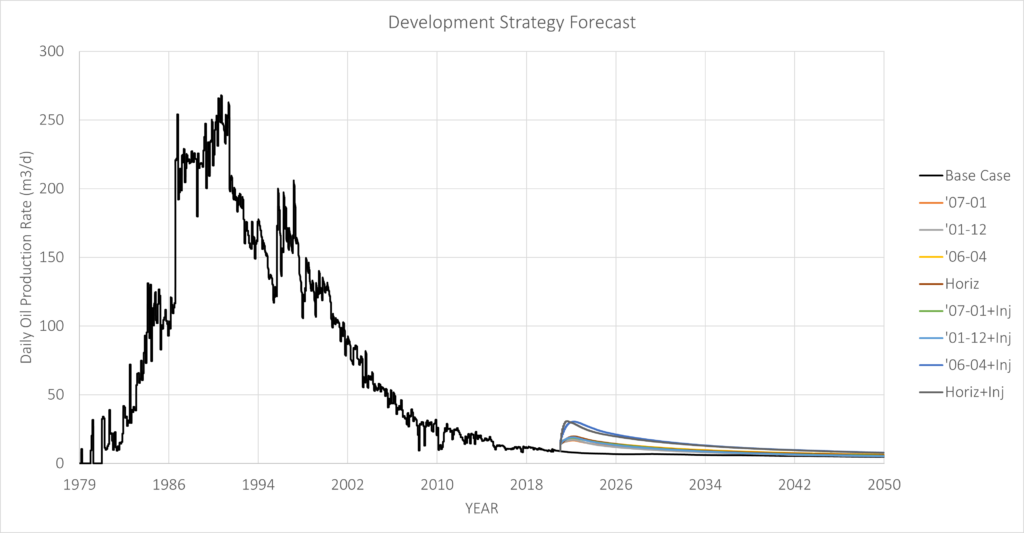
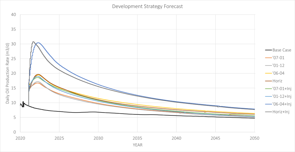
Results of the development strategy forecast are in line with what we expected. Both 07-01 and 01-12 show improved recovery from the base case and target the smaller pockets oil in their respective locations. The best recovery is seen in the development strategies targeting the eastern edge of the pool, namely reperforating well 06-04 and drilling a new horizontal well. Both of these strategies are the most effective with the extra injection in Section 5, which is logical due to the connectivity between these injectors and producers. The horizontal well was predicted to have more recovery than the existing vertical well in 06-04, so further investigation into the specifics of the well perforations, length, and location will be done to find an optimal horizontal well drilling scheme.
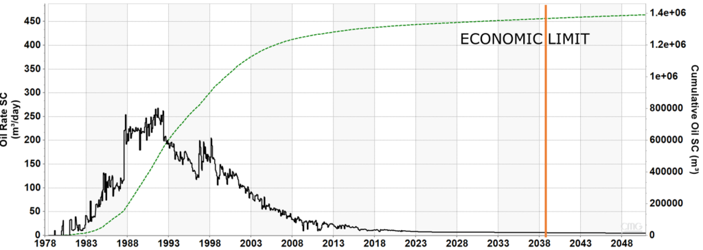
Economics
Based on the base case forecast for our pool, the NPV is calculated as $1.10 million at a 10% discount rate with an end of life of 2039. At this economic limit, the ultimate recovery is about 1.4 million m3 of oil, which gives an Ultimate Recovery Factor (URF) of 32%.
The following table details the Capital Investment (CAPEX), Net Present Value (NPV), Economic Limit, and Incremental Recovery above Base Case for each development strategy. The perforation of 06-04 and the drilling of the new horizontal well in Section 4 are the most profitable options, which is as expected due to the large pocket of oil in the eastern edge of the pool. For each of these cases, the most economically favourable method is to increase the injection rates along with reperforating or drilling the well. However, the most profitable option appears to be the perforation of well 06-04-049 with increased injection from turning on existing injectors in Section 5. This method proves to be perhaps more profitable than the drilling of the new horizontal well as it has a drastically lower capital investment.
| Case | CAPEX | NPV | Economic Limit | Incremental Recovery (bbl) |
|---|---|---|---|---|
| Base | 0 | $1.10 million | Mar-2039 | — |
| 07-01 Restart | $100k | $3.73 million | Jul-2039 | 0.165 million |
| 01-12 Restart | $100k | $3.54 million | Jul-2042 | 0.155 million |
| 06-04 Reperf. | $200k | $4.72 million | Jan-2048 | 0.267 million |
| New Horizontal | $2 million | $4.36 million | Jan 2046 | 0.241 million |
| 07-01 + Injection | $150k | $3.97 million | Mar-2042 | 0.205 million |
| 01-12 + Injection | $150k | $3.94 million | May-2042 | 0.196 million |
| 06-04 + Injection | $250k | $7.98 million | Oct-2050 | 0.546 million |
| Horizontal + Injection | $2.05 million | $7.49 million | May 2050 | 0.509 million |
Our Solution
Following the forecasts and economic analysis for each development strategy investigated thus far, the best choice would be to reperforate the lower zone of well 06-04-049 in the east and turn on both 06 and 10-05-049 injectors. Reporforating 06-04 provides access to the pocket of oil in the east without having to drill a new expensive well which saves time, money, and resources. Further investigation will be done to confirm the feasibility of this strategy as the history matching process continues to improve.
Partners and Mentors
Special thanks to our mentors this term Dr. Harvey Yarranton and Michael Aikman for all the support during this project.
Thank you also to Whitecap for providing us with valuable information and guidance.

Dr. Harvey Yarranton
Department of Chemical & Petroleum Engineering
Mentor – Academic

Dr. Michael JL Aikman, MBA
Reservoir Engineering Expert,
Upstream Technology Center,
Abu Dhabi National Oil Company
Mentor – Industry

Whitecap Resources Inc.
Pool Owner & Operator
References
[1] B. M. Jones, “Integrated Ichnology and Sedimentology of Mixed River- and Wave-Influenced Delta Complexes, Upper Cretaceous Basal Belly River Formation, Central Alberta, Canada.” Order No. MS23953, Simon Fraser University (Canada), Ann Arbor, 2013.
[2] C. D. Hansen, “Facies Characterization and Depositional Architecture of a Mixed-Influence Asymmetric Delta Lobe: Upper Cretaceous Basal Belly River Formation, Central Alberta.” Order No. MR41067, Simon Fraser University (Canada), Ann Arbor, 2007.
[3] A. Hamblin and B. Abrahamson, “Bulletin of Canadian petroleum geology”, Canadian Society of Petroleum Geologists, vol. 44, no. 4, pp. 654-673, 1996. Available: https://pubs-geoscienceworld-org.ezproxy.lib.ucalgary.ca/cspg/bcpg/article/44/4/654/57685/Stratigraphic-architecture-of-Basal-Belly-River. [Accessed 22 October 2021].
[4] “Chapter 17 – Paleographic Evolution of the Western Canada Foreland Basin”, Alberta Geological Survey, 2016. [Online]. Available: https://cspg.org/common/Uploaded%20files/pdfs/documents/publications/atlas/ geological/ atlas_17_paleogeographic_evolution_of_foreland_basin.pdf. [Accessed 22 October 2021].
[5] “Chapter 20- Cretaceous Colorado/Alberta Group of the Western Canada Sedimentary Basin”, Alberta Geological Survey, 2016. [Online] Available: https://cspg.org/common/ Uploaded%20files/pdfs/documents/publications/atlas/geological/atlas_20_cretaceous_colorado-alberta_groups.pdf. [Accessed 22 October 2021].
